Classified Urban Land Cover Classes

Classified Urban Land Cover Classes: History

Please note this is an old version of this entry, which may differ significantly from the current revision.

Subjects: Area Studies

Contributor:

remote sensing
urban environment
data fusion
sensor fusion
urban mapping
land cover classification

1. Introduction

Over the last few decades, global urbanization has grown rapidly. By 2050, around 68% of the world’s population will be living in urban areas [1]. This can cause environmental challenges, including ecological problems, poor air quality, deterioration of public health, microclimate changes leading to severe weather, higher temperatures, limited access to water, persistent vulnerability to natural hazards, and the release of toxic particles from fast industrialization into the atmosphere [2,3]. These challenges lead to difficulties in advanced urban analyses due to urban surfaces’ spectral and structural diversity and complexity over a small area [4,5]. Therefore, constant monitoring of urban areas is often highly required. Systematic monitoring and updating of maps are critical in urban areas, where many objects are mobile (vehicles and temporary buildings), and the infrastructure, vegetation, and construction are constantly changing.

Spatiotemporal investigations of the urban regions are today provided by remote sensing technology advances [6]. Especially, airborne remote sensing is a powerful developing tool for urban analysis that offers time-efficient mapping of a city essential for diverse planning [7], management activities [8], and monitoring urban and suburban land uses [9]. It has been proven as a common technique for mapping urban land cover changes to investigate, e.g., social preferences, the regional ecosystem, urbanization change, and biodiversity [10]. Urban remote sensing, in particular, is widely used for the investigation of three-dimensional urban geometry that is crucial for modeling urban morphology [11], identifying various objects, heterogeneous material, and mixtures. However, the growing challenges require a state-of-the-art technological solution in terms of sensors and analysis methods. Continuous development and improvement of remote sensing sensors increase interest in identifying urban land cover types based on spectral, spatial, and structural properties [12,13]. In urban mapping, lidar analyses (light detection and ranging), hyperspectral data (HS), and synthetic aperture radar (SAR) have become significant. Different portions of the electromagnetic spectrum are useful in analyzing urban environments from the reflective spectral range to the microwave radar [14]. The latter provide high-resolution images independent of the time of day and weather; however, due to the requirement of oblique illumination of the scene, occlusion and layover appear, making the analysis of dynamic urban areas difficult [15].

Urban land cover classification accuracy and interpretability based only on a single sensor in complex, dense urban areas are often insufficient [16]. The heterogeneity in the urban areas leads to high spectral variation within one land cover type, resulting in very complex analyses. The impervious surfaces (roofs, parking lots, roads, and pavements) notably vary in the spectral and spatial-structural manner. In addition, scale and spatial resolution are relevant for estimating urban heterogeneity. Scale defines heterogeneity, in which materials are taken into account analytically or absent or grouped into one class, e.g., individual trees, type versus forest, or vegetation in general [17]. Spatial resolution, on the other hand, determines the level of pixel mixing. However, high spatial resolution increases the physical material heterogeneity, increasing the complexity of analyses.

HS data provide spectral information about materials, differentiating them without elevation context. The challenge in the pure spectral analysis is the negligence of object identification, mostly built from various materials maintaining very high intra-object heterogeneity. By contrast, lidar data can distinguish between different land cover classes from the same material at a different height, such as asphaltic open parking lots and roads [18,19]. Furthermore, passive remote sensors, such as HS, are sensitive to atmospheric conditions and illumination, whereas lidar as an active sensor is less sensitive to these factors. This property of lidar enables, e.g., a physical correction of shadow and illumination purposes when combined with HS data [20,21,22,23,24,25] and intensity measurement for urban land cover mapping in shaded areas [26]. Regardless of the spatial and spectral resolution of airborne-based HS sensors, urban environments are characterized by spectral ambiguity and reduced spectral value under the shadow caused by topography changes, buildings, and trees, which can be overcome by adding lidar data as presented by [27].

Moreover, a fusion of spectral, spatial, and elevation features provides robust and unique information relevant to the urban environment [30]. The airborne HL-Fusion has already been investigated for urban land cover classification purposes [30,32,33]. However, diverse combination methods are implemented on different data and product levels based on either physical or empirical approaches [34]. Furthermore, since all fusion processes are very complex, there is no defined framework for fusing these sensors. Therefore, a comprehensive summary of previous research on data fusion may enhance the understanding of fusion possibilities, challenges, and common issues that limit the classification results in the urban environment.

2. Classified Urban Land Cover Classes

The urban land cover consists of very complex physical materials and surfaces that are constantly having anthropological impacts. The urban surface types are a mosaic of seminatural surfaces such as grass, trees, bare soil, water bodies, and human-made materials of diverse age and composition, such as asphalt, concrete, roof tiles for energy conservation and fire danger [50], and generally impervious surfaces for urban flooding studies and pollution [51]. The complexity of urban analysis also depends on the scale chosen and its purpose. Many classifications refer to urban materials with fine spatial resolution deepening the heterogeneity, allowing a more detailed mapping result. The classification of urban objects, which consist of many different materials and variance within a class, although significant (e.g., in city map updates), becomes a challenge due to the highly nonlinear and heterogeneous composition of different objects surfaces and materials, and thus, there is the need to use more training data for classification purposes, which is time-consuming and computationally expensive.

2.1. Buildings

Buildings in an urban context can be recognized as shapes with planar surfaces and straight lines [52]. Building detection based on remote sensing methods plays a crucial role in many applications in the urban environment, such as in 3D monitoring of urban development in time [53], urban planning, telecommunication network planning, vehicle navigation [33], urban energy planning [53], city management, and damage assessment [54]. Many mapping techniques are based on shape identification, outlines, and preliminary model data [54]. Besides detecting buildings as objects, building roof extraction has recently been a hot topic within the remote sensing community. Building roofs are defined by planarity properties and height derivatives based on elevation. A 3D visualization of buildings is of great importance for infrastructure management and modeling, 3D city mapping, simulations, change detection, and more [55]. Both airborne-based optical and lidar data have been used recently to map buildings. A common way to detect buildings is to use a digital surface model (DSM) [56,57], a normalized DSM (nDSM) [58,59], or a point cloud extracted from lidar data [60,61,62,63]. Lidar is capable of extracting building heights and planar roof faces [33]. It is beneficial for spatiotemporal assessment and investigation of building density for sustainability study and residential development in cities [53].

By contrast, airborne-based HS data can better distinguish between materials at the roof surfaces due to their spectral differences [33]. However, not including the elevation information from the lidar scanner, the classification of buildings and their roofs can be too complex without human expertise.

2.2. Vegetation

Vegetation is recognized by its geometrical complexity, defined by parameters such as the roughness, point density ratio measure [65], and chlorophyll spectral feature. In the last decade, active (Sentinel-1, LiDAR, and radar) and passive (Quickbird, Worldview, Sentinel-2, Landsat, and MODIS) remote sensing has been widely applied to vegetation detection. Lidar data are used to generate virtual 3D tree models [66], map low and high vegetation [67], and, using multispectral lidar, assess vegetation variety regarding its health and density [68], as well as extract vegetation indices, e.g., NDVI [69] for monitoring changes caused by urbanization, anthropogenetic activities, and harvesting applying wavelet transform [70,71]. However, vegetation detection is not a straightforward approach. The analysis is often complex and detailed due to the increasingly finer spatial resolution of remote sensing devices, such as distinguishing photosynthetic and nonphotosynthetic vegetation [72]. Vegetation is often not defined as a whole but as groups, for example, as low vegetation (grass), middle vegetation (shrubs), and high vegetation (trees). One of the more complex challenges is the similar morphology of low/young trees and shrubs, causing misclassification of shrubs as high trees [73]. HS data are also used to detect vegetation on a spectral basis (chlorophyll reflectance), differentiating between vegetation types and healthiness. More biophysical parameters can be defined due to more spectral bands than multispectral lidar (usually 2–3 wavelengths), such as the leaf area index, fractional cover, and foliage biochemistry [74]. Both sensors have been fused in many studies, e.g., for canopy characterization for biomass assessment and estimation of risk of natural hazards [75] and urban tree species mapping [76].

2.3. Roads

Road detection from airborne-based HS and lidar data is essential in remote sensing applications, e.g., a road navigation system, urban planning and management, and geographic information actualization [77,78]. The elevation feature derived from lidar data has been proven as a significant parameter to extract time-efficient road methods compared to optical methods [79]. DSM distinguishes more precise boundaries of surfaces, even in occluded regions [80]. However, only lidar-data-based classification is limited when roads are at the same elevation but made of different materials, such as asphalt, concrete, or other impervious materials [18]. Therefore, HS imaging can differentiate between different materials and their conditions to complement road classification purposes. It has already been proven by Herold et al. [81] for the following uses: map alteration, degradation, and structural damages of road surfaces based on spectral analysis. Usually, to detect roads, texture information is implemented [82]. In addition, lane marks can be used as an indicator for new roads; however, this approach is illumination sensitive [83]. HS data classification without topographic information is challenging when differentiating between two objects made from the same material: differentiation between a parking lot, parking at the ground level, cycleway, and a road [30].

2.4. Miscellaneous

Apart from the above-described land cover classes, the urban environment consists of more complex thematic classes. They commonly cannot be chemically or physically described by a single hyperspectral absorption feature or other single features, such as height or shape, which are, however, extracted from contextual information. Thus, spatial context is critical and necessary for identifying industrial areas, commercial or residential buildings, playgrounds, and harbors in coastal cities. The combination of spectral and spatial features from HS and lidar data shows potential, allowing identifying thematic class and assessing its condition in terms of quality and materials.

3. Key Characteristics of Hyperspectral and Lidar Data

3.1. Hyperspectral (HS) Images

HS data retrieved from an imaging spectrometer are a three-dimensional cube that includes two-dimensional spatial information (x, y) with spectral information at each pixel position x_iy_j [87]. Each pixel in the obtained digital data contains a nearly continuous spectrum covering the reflective spectral range of the visible, near-infrared (VNIR: 400–1000 nm) and short-wave infrared (SWIR: 1000–2500 nm) [88,89]. HS as a passive system is dependent on the given lighting conditions resulting in high intraclass (within a class) spectral variability. In these wavelength ranges of the electromagnetic spectrum, particular absorption features and shapes make it possible to identify the material’s chemical and physical properties [90].

3.1.1. Spectral Features

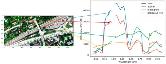
Within one material, spectral features can vary due to color, coating, degradation, alteration, roughness, the illumination of material, data acquisition, location of the material, and preprocessing data (Figure 2) [97,107,108]. These variations within a material are more and more investigated, generating spectral libraries of complex urban materials [12,109,110] and normalization based on advanced preprocessing. HS images result in high-dimensional data leading to computationally expensive analyses.

Figure 2. At surface reflectance of some urban surfaces (HySpex sensors VNIR-1800 and SWIR-384). The hyperspectral dataset was acquired by the Terratec AS Company in August 2019 over Baerum municipality, Oslo, Norway.

3.1.2. Spatial Information

Spatial-context information is widely used to achieve robust and accurate classification maps considering the neighborhood in the target pixel. While spectral features are the most relevant features in material-based classification, adding spatial features to object classification makes it easier to group pixels with some spectral variance into one class representing an object or land cover type [126]. In addition, the spatial noise of the classification results can be reduced [127,128].

3.2. Lidar Data

Lidar data is a three-dimensional point cloud (x, y, z) which delivers by default information about elevation, multiple-return, the reflected intensity, texture, and waveform-derived feature spaces from the object hit by laser pulse [31,134]. As an active sensor, a lidar system emits radiation from one bandwidth (more in the case of multiwavelength lidar scanners) to the object surface at high repetition rates. Lidar scanners are whiskbroom-type instruments and typically use the monochromatic laser in visible—532 (bathymetric/coastal mapping)—and near-infrared—1064 and 1550 nm—for example, for vegetation detection and differentiation between asphaltic and nonasphaltic roads [135] which can be used as an additional intensity feature in land cover mapping in the reflective spectral range [31]. The advantage of using airborne lidar is insensitivity to relief displacement and illumination conditions [31], retaining full 3D geometry of data.

3.2.1. Height Features and Their Derivatives (HD)

The height feature is used to calculate the three-dimensional coordinates (x,y,z) that generate a gridded 2.5-dimensional topographical profile of the area of interest [31]. Especially in the urban environment, the z value height is crucial for precise contour generation of elevated objects [31]. 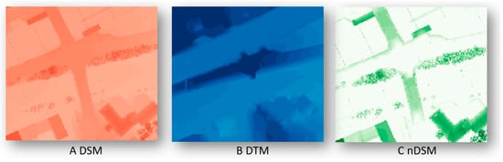In addition, the height difference between the lidar return and the lowest point in cylindrical volume has been investigated and proven as an important feature in discriminating ground and nonground points [136,137]. Moreover, a digital surface model (DSM) (Figure 3A) is extracted from the height information applying interpolation of 3D points onto a 2D grid. From a DSM, a surface roughness layer [138] and a normalized DSM (nDSM) (Figure 3C) are calculated, subtracting the digital terrain model (DTM) (Figure 3B) from the DSM [31]. The overlapping of the building height information and the terrain height information is thus excluded. The object representation heterogeneity is therefore reduced, which helps the classification procedure.

Figure 3. Examples of DSM (A), DTM (B), and nDSM (C) from Riegl VG-1560i LiDAR scanner acquired by the Terratec AS Company in August 2019 over Baerum municipality, Oslo, Norway.

3.2.2. Intensity Data

Intensity values extracted from lidar data correspond to the peak amplitudes from the illuminated object [31]. Applying intensity as a feature space, Song et al. [148] presented an approach to determine asphalt roads, grass, house roofs, and trees. However, trees’ diverse intensity values undermine the classification due to the canopies’ complex geometry [149].

3.2.3. Multiple-Return

A lidar-based laser pulse can split into multiple laser returns if it hits a permeable object such as a tree canopy and obtains a response from, e.g., branches, leaves, stems, and the ground [31]. Multiple-return data has been recently used as an additional feature space in the urban mapping in the commercial building, small house, and tree determination [146].

3.2.4. Waveform-Derived Features

Full-waveform lidar scanners can retrieve the entire signal of the backscattered laser pulse as a 1D signal profile in the chronological sequence [134,156,157]. A full-waveform lidar system can better correct the intensity values than the discrete systems, such as accurate estimation of the surface slope [158], eliminating the assumption of Lambertian reflectors [159]. However, before using any classification approach, proper radiometric calibration is needed to adjust waveform data from different flight campaigns.

3.2.5. Eigenvalue-Based Features

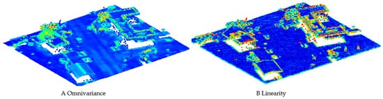
The eigenvalues are calculated based on the covariance matrix of x, y, and z dimensions of the 3D point cloud as λ₁, λ₂, and λ₃. Eigenvalues as features help detect geometrical parameters, such as plane, edge, and corner [171]. The following structure features have been applied to lidar data: omnivariance, anisotropy, planarity, sphericity, linearity, and eigenentropy for features for context-driven target detection [172] building detection [171]. Some of them are shown in Figure 5. The planarity feature is proven relevant for road classification or other flat surfaces and sphericity for building and natural ground (low vegetation) detection [136].

Figure 5. Structure features derived from lidar data: omnivariance (A) and linearity (B) from [171].

3.3. Common Features—HS and Lidar

3.3.1. Textural Features

Besides spectral information of hyperspectral sensors, pixel-wise spatial features are relevant for image content, such as textural features. The textural attributes in a hyperspectral scene can be extracted by the local binary patterns (LBP) operator proposed by [173], providing information about the surface granularity [174]. To include spatial information in the classification purposes, the textural operators are window based. Peng et al. [175] extracted them as rotation-invariant features for urban classification purposes except for spectral features and Gabor features [176]. The latter are frequential filters interpreting the texture of the hyperspectral bands used by [177,178]. The texture can be analyzed by applying the gray-level co-occurrence matrix (GLCM) measures [53,179].

3.3.2. Morphological Features

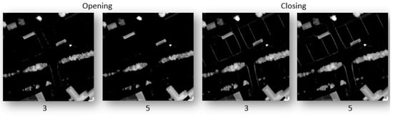
Mathematical morphology contains operators such as erosion, dilation, opening, closing, rank filters, top hat, and other derived transforms. Mainly, these operators are applied on panchromatic images from hyperspectral sensors, binary or greyscale images with isotropic and geodesic metrics with a structural element [185]. For example, the opening operator focuses on the bright spots, removing objects smaller than the structural element, whereas the closing operator acts on the dark objects (Figure 6).

Figure 6. Opening and closing operations on lidar dataset with different kernel sizes (3 and 5) of the structural element.

3.4. Hyperspectral-Lidar Data Fusion

HL-Fusion combines spectral-contextual information obtained by an HS sensor and a lidar scanner’s spectral-spatial-geometrical information. Even if the active and passive sensors characterize different physics, their features can be combined from both sensors. Both sensors cover the reflective spectral range intersecting either in the VIS (532 nm) or the SWIR (1064, 1550 nm) wavelength regions. More rarely, multi-spectral lidar systems are used, which overlap in several of the three common wavelengths, allowing the identification of materials or objects using spectral properties [194]. Under laboratory conditions, prototypical hyperspectral lidar systems are being developed [69,195,196].

This entry is adapted from the peer-reviewed paper 10.3390/rs13173393

© Text is available under the terms and conditions of the Creative Commons Attribution (CC BY) license; additional terms may apply. By using this site, you agree to the Terms and Conditions and Privacy Policy.