Using observational data covering 1948–2020, the environmental factors controlling the winter precipitation in California were investigated. Empirical orthogonal function (EOF) analysis was applied to identify the dominant climate regimes contributing to the precipitation. The first EOF mode described a consistent change, with 70.1% variance contribution, and the second mode
exhibited a south–east dipole change, with 11.7% contribution. For EOF1, the relationship was positive between PC1(principal component) and SST (sea surface temperature) in the central Pacific Ocean, while it was negative with SST in the southeast Indian Ocean. The Pacific–North America mode, induced by the positive SST and precipitation in the central Pacific Ocean, leads to California
being occupied by southwesterlies, which would transport warm and wet flow from the ocean, beneficial for precipitation. As for the negative relationship, California is controlled by biotrophically high pressure, representing part of the Rossby wave train induced by the positive SST in the Indian ocean, which is unfavorable for the precipitation. For EOF2, California is controlled by positive
vorticity at the upper level, whereas at the lower level, there is positive vorticity to the south and negative vorticity to the north, the combination of which leads to the dipole mode change in the precipitation.
1. Introduction
The state of California is the largest agricultural producer of the United States (US) and one of the major agricultural areas of the world [
1,
2]. According to the survey, it accounts for a greater share of the population, cash farm receipts, and gross domestic product [
3,
4,
5] than other states in the US.
In recent decades, the frequency of floods and droughts in the US has increased [
6]. For example, the persistent droughts in the summers of 2002 and 2007 posed a considerable threat to water resources [
7], and the record-breaking floods in Georgia in September 2009 destroyed thousands of homes and caused huge losses [
8]. More recently, California suffered a multiyear drought. For example, 2012–2014 featured the worst drought in the region in the past 1200 years, with soil moisture persistently below average [
9]. Although global warming caused by human activities accounts for 5–18% of the abnormal droughts, natural variability is still the main controlling factor for the precipitation anomaly [
10,
11]. Due to the important location of California and because the abnormal precipitation level determines the extent of drought or flood disaster, which then influences the agriculture and socioeconomics, it is critical to analyze the rainfall anomaly in California.
A number of previous studies has investigated the precipitation in summer in the US. For example, they proposed that convective heating over the subtropical western Pacific Ocean could induce a wave train pattern, which spans the northern Pacific Ocean and North America, affecting US precipitation [
12,
13,
14]. Through further analysis, it was pointed out that this wave train may stem from marginally unstable normal modes of the summertime large-scale monsoon circulation [
15]. During the great floods of 1993 in the US Midwest, pronounced sea surface temperature (SST) signals in the subtropical North Pacific and tropical eastern Pacific Ocean were found [
16,
17]. In recent years, strong tele-connection signals emanating from the subtropical northwestern Pacific Ocean through the Aleutians to North America during the stronger Asian monsoon activity periods have been emphasized [
18,
19,
20]. Simultaneously, many studies have confirmed the important role of remote forcing in causing precipitation anomalies over the US over a wide range of time scales [
21,
22,
23,
24,
25]. The literature suggests that the variability of the US summer rainfall may not only be governed by the Pacific Ocean SST anomalies [
16,
21,
26,
27,
28,
29,
30], but also be attributable to Atlantic Ocean SST anomalies [
31,
32,
33,
34,
35].
Some studies have also shown a close link between the US winter rainfall variability and the Pacific Ocean–North America (PNA) teleconnection pattern [
36,
37,
38,
39,
40]. Coleman and Rogers (2003) [
41] pointed out that the PNA pattern had significant negative correlations with winter precipitation over the Ohio River Valley. During negative PNA winters, moisture flux convergence extended much further north from the Gulf of Mexico and brought more precipitation. Ge et al. (2009) [
42] showed that the PNA pattern also influenced snow conditions over portions of North America through its influence on both winter temperature and precipitation.
Even though previous studies have mentioned the possible mechanism underlying US precipitation, few have focused on winter precipitation in California to identify impact factors in the leading time. In addition, to prepare for climate predictions, atmospheric signals, with physical meanings, in the leading time are needed for precipitation forecasts. The objective of the current study was to investigate the environmental factors controlling precipitation in the winter in California. The remainder of this paper is organized as follows: in
Section 2, the data and analysis method are introduced. The basic mode of California precipitation is shown in
Section 3. The environmental factors affecting PC1 and PC2 changes are described in
Section 4 and
Section 5. Lastly, a summary and discussion are given in
Section 6.
2. Environmental Factors Affecting PC1 Changes
Since EOF1 and EOF2 described two different processes, the changes in PC1 and PC2 were analyzed separately.
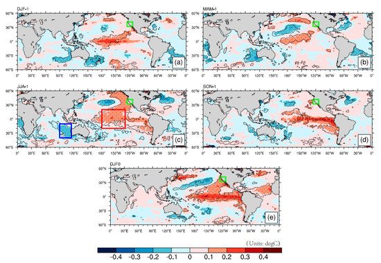
Figure 3 shows the evolution of SST patterns regressed to PC1 from the preceding winter to the subsequent winter. In both winters, we can see an El Niño-like pattern, which indicates that warm SST in the eastern Pacific Ocean corresponded to positive precipitation in California, consistent with previous studies [
54]. It is worth noting that the positive relationship was continuous from the preceding winter to autumn. As the predictions of drought and flood are often needed one season in advance, and the signal in the preceding summer was most significant, the environmental factors were chosen in the preceding summer, as shown in
Figure 3c. There was a positive relationship between SST in the central Pacific Ocean (red box; 20° S–20° N; 180–130° W) and California precipitation, as well as a negative relationship between SST in the southeast Indian Ocean (blue box; 40–10° S; 90–115° E) and California precipitation.
Figure 3. Evolution of SST patterns (°C) regressed to standardized PC1 from the preceding winter (a) to spring (b), summer (c), autumn (d) and the subsequent winter (e). Areas with dots exceed a 90% confidence level. The green box represents the selected California area. Red and blue boxes denote key regions analyzed.
3. Environmental Factors Affecting PC2 Changes
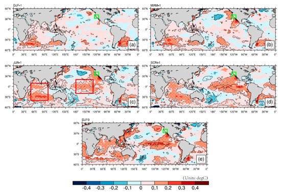
Figure 9 shows the evolution of SST patterns regressed to PC2 from the preceding winter to the subsequent winter. In both winters, we can see an El Niño-like pattern, which indicates that warm SST in the eastern Pacific Ocean corresponded to positive precipitation in California. Other than the decreased level of relevance, this characteristic was similar to PC1; thus, the environmental factors in the Pacific Ocean are not discussed here.
Figure 9. Same as in Figure 3, except for PC2.
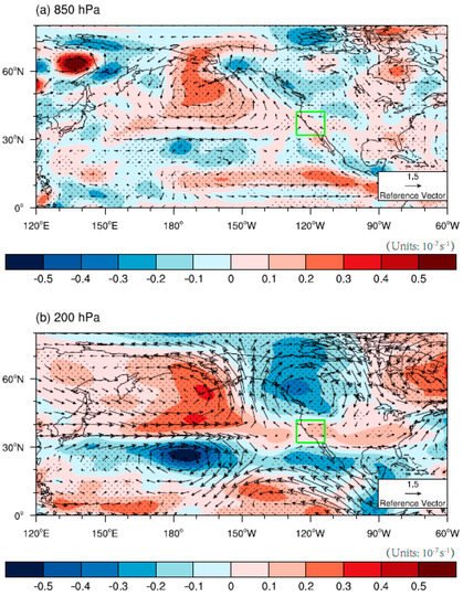
The situation was different in the Indian ocean. The relationship between PC2 and SST in the Indian Ocean in the preceding summer was significantly positive. In order to determine how the SST in the Indian Ocean influences California precipitation, index 3 was defined as the average SST in the mostly positive related region (40° S–10° N; 50–100° E; left red box in Figure 9c) in the preceding summer. Figure 10 shows the relative vorticity and horizontal velocity at 850 hPa and 200 hPa in winter regressed to index 3. From the figure, we can see that, at the upper level, the key region is controlled by positive vorticity and a cyclone, whereas at the lower level, the situation is complex. In the south of California, there is positive vorticity. Combined with circulation at the lower level, such positive vorticity is beneficial for positive precipitation. On the other hand, in the north of California, there is negative vorticity, which is unfavorable for precipitation. As a result, the combination of upper and lower circulation is favorable for precipitation in the south but unfavorable in the north, leading to a dipole mode of precipitation, which is consistent with EOF2.
Figure 10. Relative vorticity (shading; 10−7 s−1) and horizontal velocity (vector; m/s) at 850 hPa (a) and 200 hPa (b) in winter regressed to the box-averaged SST (the left red box in Figure 9c). The green box represents the selected California area. Areas with dots exceed the 90% confidence level.
4. Summary and Discussion
In this study, the environmental factors affecting precipitation in California during 1948–2020 were investigated. Considering the seasonal mean and standard deviation of precipitation, this paper focused on winter as the main rainy season with the greatest variation. According to the EOF analysis of winter precipitation, the first EOF mode described a consistent change, with a variance contribution of 70.1%. The second EOF mode exhibited a south–east dipole change with an 11.7% variance contribution.
For EOF1, the relationship was positive between SST in the central Pacific in the preceding summer with PC1 in winter and negative between SST in the southeast Indian Ocean in the preceding summer with PC1 in winter. Due to the slow change and continuity of SST, the warm SST in the central Pacific Ocean would be maintained from summer to winter. Thus, the positive precipitation induced would exist in the subsequent winter in the central Pacific Ocean, thereby inducing a PNA-type wave train response to influence the California precipitation. Regardless of whether the lower level or the upper level was considered, the key region was located to the southeast of the anomalous cyclone induced. The southwesterly wind would transport warm and wet flow from the ocean, beneficial for precipitation. There is another possible process underlying how warm SST in the central Pacific Ocean would affect California precipitation. California is located around the boundary of the tropical belt, at the edge of the Hadley cell sinking phenomenon. The edge of Hadley cells features a hot and dry climate. Yang et al. (2020) [
58] proposed that poleward shift of the meridional temperature gradients would cause expanding tropics. Therefore, the El Nino-like pattern in EOF1 favors an equator contraction of the meridional temperature gradient, contributing to a narrower Hadley cell, which is then favorable for California precipitation. For the Indian ocean, the positive SST would induce an anomalous cyclone at the lower level and an anticyclone at the upper level in the northern Indian Ocean according to the Gill response. This was confirmed by both the observation and the AGCM model experiments. Following an anomalous heating in the eastern Indian Ocean in the model, there was a cyclone anomaly response at the lower level and an anticyclone anomaly response at the upper level in the northwest. The induced Rossby wave train extends from the Indian Ocean to the Atlantic Ocean. The key region is controlled by the biotrophically high pressure, which is unfavorable for precipitation.
As for PC2, the situation in Pacific Ocean was similar to that for PC1. There was a positive relationship between SST in the central Pacific Ocean in the preceding summer and California precipitation in winter. However, the circumstances were different in the Indian Ocean, whereby the relationship between SST in the Indian Ocean in the preceding summer and California precipitation in winter was also positive. Due to the slow change and continuity of SST, the warm SST would be maintained from summer to winter, which would induce a Rossby wave train from the Indian Ocean to California. Since the key region of the Indian Ocean is shifted westward, the wave train is shifted correspondingly. As a result, at the upper level, California is controlled by positive vorticity, whereas at the lower level, there is positive vorticity in the south and negative vorticity in the north. This combination of circulation at the upper and lower levels would lead to a dipole mode of precipitation, positive in the south and negative in the north.
It is worth mentioning that, in this study, how the summer conditions affect winter precipitation was mainly attributed to the slow change and continuity of SST. However, other possibilities, such as human activities, should be considered. Furthermore, only the effect of SST in the preceding summer was analyzed. Other environmental factors, such as geopotential height, in other seasons, such as in the preceding autumn, should also be considered. In this study, we only used AGCM to confirm the physical processes. Other models, such as ECHAM, should be applied. Further studies are needed to solve these questions. Having now found the precursor signals, further studies are needed to determine whether they can be adopted in precipitation forecasts.
This entry is adapted from the peer-reviewed paper 10.3390/atmos12080997