2.1. Berlin: Balancing Demand and Yield
German per capita (PC) consumption of fresh and processed tomatoes was 27.2 kg in 2018/19, with processed tomatoes converted to fresh weight [
68]. Regarding the import and domestic harvest of fresh tomatoes, we concluded that fresh tomatoes had a share of 9.3 kg/PC and processed tomatoes 17.9 kg/PC in 2019 based on data from BLE [
69]. For freshwater fish, the shares was 3 kg/pC and 0.9 kg/PC for freshwater fish products [
70]. These data were not available for Berlin and so we assumed a similar consumption pattern to estimate the demand of metropolitan Berlin by adding the non-marketable portion, e.g., waste from fish processing. With a population of about 3.77 million in 2020 [
71], approximately 21 kilotonnes (kt) of freshwater fish and fish products, 108 kt of fresh tomatoes and tomato products, and 27 kt of lettuce are required per year (cf.
Table 2).
Table 2. Annual metropolitan Berlin demand for freshwater fish/fish products, tomatoes/tomato products (converted to fresh weight), and lettuce.
The following proportions of AP setups have been calculated: catfish/tomato at 56%, catfish/lettuce at 13%, tilapia/tomato at 31%, and tilapia/lettuce at 0% (cf. Table 3). Berlin’s F/P demand ratio was around 6.5, while the F/P ratio of AP setup AP4 (tilapia/lettuce) was 56.2; therefore, its proportion was set to zero (cf. Table 4).
Table 3. Upscaled-AP scenario: Four aquaponic setups as combinations of catfish/tilapia and tomato/lettuce and their respective share to meet the freshwater fish demand of Berlin.
Table 4. Upscaled-AP scenario: The proposed annual yield of catfish, tilapia, tomato, and lettuce per aquaponic setup; Number of AP facilities required to achieve this yield.
2.2. Supply-Side: Impact on Berlin FWE Nexus
Food. The yield shares (fish/crop) of each AP setup within the upscaled-AP scenario to cover the city’s demand are as follows: AP1 with 11.5 kt catfish and 37.5 kt tomato, AP2 with 2.7 kt catfish and 27.3 kt lettuce, and AP3 with 6.3 kt tilapia and 70.9 kt tomato (cf. Table 4).
In order to produce a yield of 20.6 kt fish and 108.4 kt crop (tomato and lettuce) per annum, approximately 370 AP facilities are needed and this requires a total area of 224 hectares (cf. Table 4). Fish feed and fertiliser should ideally be matched to the specific AP setup. The three AP configurations should be standardised to obtain the appropriate quantities of optimised fish feed and fertiliser needed to achieve economies of scales for the upscaling-AP scenario.
Water. In the present study, we extrapolated the so-called water footprint, i.e., the LCA impact category water consumption (WCO in Table 5) from the package level to the city scale. Compared to the WCO of the German market mix for fresh tomatoes and lettuce, the aquaponic production of both fresh vegetables for Berlin would save about 2.0 million cubic metres of water.
Table 5. Upscaled-AP scenario: Reduced impact of fresh tomato and lettuce production on three LCA impact categories; author’s work and the calculation based on data from comparative-LCA [
41].
Regarding the LCA impact category water scarcity (WSI), about 1.4 million cubic metres of water would be saved, especially in the Almeria region of Spain where the rapid development of greenhouse horticulture has dramatically affected the availability of groundwater resources [
72].
Energy. Replacing the German market mix of tomato or lettuce (Mix-DE) with an optimised aquaponic scenario (rooftop-APDAPS-R+) would reduce the long-term CO
2 footprint (GWP100 in
Table 5) by 7691 t CO
2-equivalents. This result can be significantly improved by using aquaponics-integrated microgrids (so-called smarthoods) where all FWE flows are circularly connected [
73].
Based on data from the comparative-LCA, the relative change in environmental impact between the scenarios Mix-DE and rooftop-AP shows a reduction in the environmental footprint for all 12 LCA impact categories (cf. Figure 2).
Of the 12 LCA impact categories, the FWE sector energy is represented by the impact categories GWP20 and GWP100, while the impact categories water consumption (WCO), water scarcity (WSP), and freshwater eutrophication (FEP) represent the sector water. The long-term CO2 footprint (GWP100) is reduced by 9% for tomatoes and 50% for lettuce. For water consumption, the reduction is even more significant and becomes negative in the analysis of the comparative-LCA (cf. Figure 2).
2.3. Causalities: Aquaponic Variables and Production-Location Shift
Upscaling urban AP triggers two FWE interactions simultaneously: (1) local food production is increased and thus (2) the relocation of production occurs. Both processes result in interactions within the FWE nexus and the associated effects become relevant for the system as a whole. Thus, all causal dependencies take effect: on the local level, since AP internals and location issues gain importance due to local resource demand; and on the global level, since upscaling the shift in production-location impacts all sectors of the FWE nexus.
In order to understand the impact of AP on the three sectors of the FWE nexus, we identified significant AP variables and examined their causal relationships (cf. Table A1), which are often mediated by other variables and results in causal chains (cf. Figure 3). However, neither the complete functional scheme of an AP nor processes outside the AP system boundary (except for phosphorus) are considered when examining these AP-internal causal chains. For example, the AP nutrient coupling degree reduces fertiliser consumption, but the environmental impacts of the production and transport of the fertiliser are not considered in the causalities unlike in the comparative-LCA.
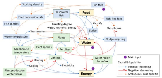
Figure 3. Impact of causal chains—formed by significant aquaponic variables—on FWE-Nexus (no flow chart; no functional scheme of an AP); the variables are explained in Table A1.
The variables listed in Table A1 influence the three sectors of the FWE nexus directly or via causal chains. These are the variables through which the designer/operator of an AP can influence the environmental impacts. General factors for increasing energy efficiencies such as solar panels, low-energy greenhouses, or energy-efficient pumps are not included in the scope of this consideration but must be taken into account as part of an overall concept. Ideally, this concept then considers future GHG attributions next to the current ones. Future GHG emission changes are expected to result from the process of decarbonisation, such as a changed electricity mix or biogas-fuelled combined heat and power unit (CHP). Figure 3 is a graphical representation of the causal chains formed by the AP variables.
The connectors in Figure 3 are causal links, but can easily be confused with flows. For example, the variable ‘plants’ affects the variable ‘water’ in that water demand increases with the number of ‘plants’, but the water needed flows from RAS to HP. We adopted the syntax of causal loop diagrams and extended it by adding case-specific considerations (ambiguous) that can results in positive or negative link polarity. The FWE nexus influences the AP parameters and creates causal loops, but these are beyond the scope of this study.
As local food production increases, the location of production simultaneously shifts across national borders. This fact touches on the problem of domestic and imported resource use and is, thus, a system boundary problem.
For example, the emission of greenhouse gases (GHG), for which its impact is indicated as GWP in the LCA approach, is an essential indicator for measuring climate sustainability. However, a country-specific CO
2 balance has some weaknesses: Germany emitted an estimated total of 805 Mt CO
2 equivalents in 2019, but almost as much (an estimated 797 Mt CO
2 equivalents) was emitted in the production of German imported goods in 2015 [
74]. Offshoring environmental damages were also criticised concerning Europe’s Green Deal [
75], but, currently, the EC 2021 proposals for making the EU’s policies fit for reducing net greenhouse gas emissions by at least 55% by 2030 [
76] include a carbon border adjustment mechanism [
77].
Comparably, local food production increases local resource use and thus impairs the ‘local ecological footprint’ while simultaneously reducing the footprint of distant production and possibly the overall ecological footprint.
The same applies to the water sector. A significant proportion of the tomatoes consumed in Berlin are produced on the Spanish Almeria peninsula around the town, El Ejido. In this region, the rapid development of greenhouse horticulture since the 1950s has dramatically affected the availability of groundwater resources [
78], which causes aquifer overexploitation. In addition, water quality deterioration occurs due to an increase in water salinity in aquifers as a result of marine intrusion processes and unsustainable aquifer management [
72]. However, the share of water needed under these troublesome circumstances to cultivate tomato for export to Germany does not appear in the German water consumption statistics.
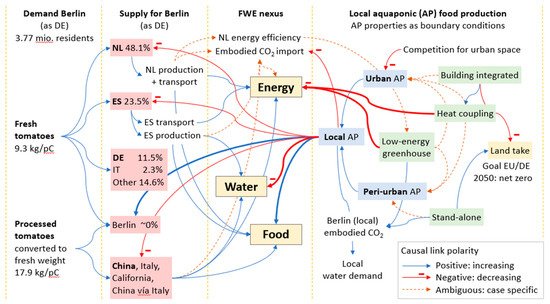
This study examines the boundary conditions for a production-location shift from other countries to Berlin based on year-round production. Compared to fish and lettuce, tomatoes have the quantitatively highest share of food production in the upscaled AP scenario (cf. Table 4), which is why tomato production is used to illustrate the dependencies of a production shift to Berlin as visualised in Figure 4.
Figure 4. Impact of simplified causal relations on the FWE nexus concerning year-round tomato production and aquaponic setup as boundary conditions for production-location shift; FWE ranking was conducted according to the main dependencies of the sectors; swim lanes are explained in Table 6.
Figure 4 contains subdivisions such as the so-called swim lanes which are explained in more detail in
Table 6. The swim lane ‘local AP’ comprises urban and peri-urban AP, as they are both within the system boundaries of the circular city (CC). Baganz et al. [
79] noted the potential for integrating AP into the CC through resource streams such as greywater, plant leftovers, and sewage; the diagram element ‘heat coupling’ in
Figure 4 is related to this.
Table 6. Causal relations of significant tomato production-location variables.
In terms of global environmental impacts and only these are considered in this study; relocation of production only makes sense if it reduces these impacts.