Your browser does not fully support modern features. Please upgrade for a smoother experience.
Please note this is an old version of this entry, which may differ significantly from the current revision.
Compact Muon Solenoid (CMS) detector and the methodology of modelling the heterogeneous CMS magnetic system for describing the magnetic flux of the CMS superconducting solenoid enclosed in a steel flux-return yoke.
- electromagnetic modeling
- magnetic flux density
- superconducting magnets
- scalar magnetic potential
- boundary conditions
1. Introduction
The discovery of the Higgs boson [1][2][3] with a mass of 125 GeV/c2 became possible due to an observation of the signals in two decay channels of this particle produced in proton–proton interactions. The first channel with a probability of 0.2% [4], is the decay channel of the Higgs boson (H) [5][6][7] into two gamma rays: H→γγ. This signal is hardly distinguished from the prevailing background of the numerous electromagnetic decays of hadrons. The second decay channel, called “gold”, is a 2.7% [4] probability decay of the Higgs boson into two Z bosons, one of which is virtual, with their subsequent decays into two oppositely charged leptons each: H→ZZ*→4l. In this case, by leptons l we mean electrons (positrons) e and muons µ. In the Higgs boson invariant mass reconstruction, four-momenta of leptons are used. This requires not only measuring the three-dimensional momenta of leptons, but also a reliable identification of these particles.
In modern detectors at circular accelerators, in particular at the Large Hadron Collider (LHC) [8], the precision tracking detectors placed in a magnetic field are used to measure momenta of the charged secondary particles generated in the interactions of the accelerated primary particle beams. The magnetic field gives to the particle trajectories in the tracking detector a curvature [9], which depends on the magnetic flux density B. A higher magnetic flux density provides a larger curvature and, as a result, a more accurate measurement of the momentum of a charged particle. Electrons and muons are identified using other systems of the experimental setup—an electromagnetic calorimeter and a muon spectrometer [10][11]. As a rule, the superconducting solenoids with a central magnetic flux density of 2–4 T [12][13][14][15][16][17][18][19] are used to create a magnetic field in modern experimental setups at the circular colliders.
During the preparation of proposals for multi-purpose experiments [20][21][22][23][24] on the search for new particle phenomena at the circular colliders with the centre-of-mass energies of colliding beams of 6–14 TeV, the processes of the Higgs boson production with a mass of up to 1 TeV/c2 with its decay into leptons in the final state were studied [25][26][27][28]. For a given mass of the Higgs boson, the statistical significance of the signal from its production remains constant in the region of transverse lepton momenta of 50–100 GeV/c. Therefore, the measurement of the lepton momentum in this region should occur in a tracking detector with a high accuracy. It was shown that the experimental resolution across the transverse momentum of a charged particle is not only directly related to the magnetic flux density in the volume of the tracking detector, but also is determined by the degradation of the double integrals of the magnetic field along the particle paths in the extreme regions of the cylindrical volume of the tracking detector [29][30].
Modern magnetic systems of multi-purpose detectors at the circular colliders are mostly heterogeneous [18][19][31][32], i.e., the magnetic flux they create penetrates both non-magnetic and ferromagnetic materials of the experimental setup. The steel yoke of the magnet is used, as a rule, as magnetized layers wrapping muons, which makes it possible to identify them and measure their momenta in a muon spectrometer. In a solenoidal magnet, the large volume of steel yoke around a coil and the inhomogeneity of the magnetic flux density in the yoke make direct measurements of the magnetic field inside the yoke blocks difficult. Existing methods for measuring the magnetic field using Hall sensors or nuclear magnetic resonance (NMR) sensors are successfully applied within the volume of the solenoidal magnet and provide a high measurement accuracy. To use such sensors in measurement of the magnetic flux density B inside the blocks of the magnet steel yoke, thin air gaps cutting the blocks in planes perpendicular to the magnetic field lines are needed. This greatly complicates the yoke as a supporting structure. An alternative option is to use a magnet current ramp down from the operating value to zero and to integrate over time the electrical signals induced by changes in the magnetic flux in sections of special flux loops installed around the yoke blocks. In the latter case, as a result of integration, the initial average density of the magnetic flux in the cross section of the flux coil can be reconstructed.
Both options allow only discrete measurements of the magnetic flux distribution in the magnet steel yoke. These are insufficient to measure muon momenta in a muon spectrometer. A computing modelling of the magnetic system to obtain the distribution of the magnetic flux throughout the entire experimental setup achieves this goal.
2. The CMS Detector Description
In the Compact Muon Solenoid (CMS) detector [11] at the LHC [8], the magnetic field is provided by a wide-aperture superconducting thin solenoid [33] with a diameter of 6 m and a length of 12.5 m, where a central magnetic flux density |B0| of 3.8 T is created by an operational direct current of 18.164 kA [34][35][36]. The CMS multi-purpose detector, schematically shown in Figure 1, includes a silicon pixel tracking detector [37], a silicon strip tracking detector [38], a solid crystal electromagnetic calorimeter [39] to register e and γ particles, and a hadron calorimeter of total absorption [40] both located inside the superconducting solenoid, as well as a muon spectrometer [41][42][43][44] and a forward hadron calorimeter [45], both located outside of the superconducting coil. One of the main goals of the CMS setup was to detect the Higgs boson by its decay mode into four leptons H→4l, where l = e, µ, and the technical design of all the detector systems has led to the success in achieving this purpose.

Figure 1. Schematic view [46] of the CMS detector in transverse (a) and longitudinal (b) sections. Designations are as follows: S1–S12—the detector azimuthal sectors; TC and L1–L3—layers of the yoke barrel wheels (W); D—the yoke endcap disks; Chimneys—grooves in the barrel wheels W + 1 and W − 1 for pipelines of the cryogenic system and current leads of the solenoid (COIL), respectively.
The heart of the CMS detector — magnetic system comprises a NbTi superconducting solenoid and a magnetic flux return yoke made of construction steel containing up to 0.17% carbon and up to 1.22% manganese, as well as small amounts of silicon, chromium, and copper. The solenoid [34], creating a magnetic flux of 130 Wb, is installed in a vacuum cryostat in the central four-layer barrel wheel of the magnet yoke [35]. The magnet yoke also includes two three-layer barrel wheels around the solenoid cryostat on each side of the central barrel wheel, two nose disks inside each end of the solenoid cryostat, and four endcap disks on each side of the cryostat.
The inner diameter of the solenoid cryostat is 5.945 m, the diameter of each nose disk is 5.26 m, the inscribed outer diameters of the 12-sided barrel wheels around the cryostat are 13.99 m, the inscribed outer diameters of the 12-sided endcap disks are 13.91 m, the length of the magnet yoke is 21.61 m, and the weight of the magnetic flux return yoke is more than 10,000 tons. There are two halves of the forward hadron calorimeter, and two radiation shields around the vacuum beam pipe downstream of the endcap disks on each side of the yoke at 10.86 m off the solenoid centre. The total thickness of steel along the radius of the central barrel wheel is 1.705 m, the total thickness of the endcap disks on each side is 1.541 m, and the thickness of each nose disk is 0.924 m.
Only two thirds of the solenoid magnetic flux passes through the cross sections of the magnet yoke. The remaining third of the magnetic flux creates a stray magnetic field around the magnet yoke, the value of which decreases with a radius around the solenoid axis and with a distance along the axis. At a radius of 50 m from the coil axis in the central plane of the detector, the value of the magnetic flux density is 2.1 mT. At a distance of 50 m from the centre of the solenoid along its axis, the value of the magnetic flux density becomes 0.6 mT. The contribution of the barrel wheels, nose, and endcap disks to the central magnetic field is 7.97%, the contribution of the steel absorber of the forward hadron calorimeter, ferromagnetic elements of the radiation shielding, and the 40 mm thick steel floor of the experimental underground cavern is only 0.03%.
The CMS detector provides registration of charged particles in the pseudorapidity region |η| < 2.5, registration of e and γ in the region |η| < 3, registration of hadronic jets in the region |η| < 5.2, and registration of µ in the region |η| < 2.4 [11]. The pseudorapidity η is determined as η = −ln[tan(θ/2)], where θ is a polar angle in the detector reference frame.
The origin of the CMS coordinate system is located in the centre of the superconducting solenoid, the X axis lies in the LHC plane and is directed to the centre of the LHC machine, the Y axis is directed upward and is perpendicular to the LHC plane, and the Z axis makes up the right triplet with the X and Y axes and is directed along the vector of magnetic induction created on the axis of the superconducting coil.
Until 2013, a pixel tracking detector [37] consisted of 1440 silicon modules; a strip tracking detector [38] consists of 15,148 silicon modules. Both tracking detectors provide a resolution in the impact parameter of charged particles at a level of ≈15 μm and a resolution in the transverse momentum pT of charged particles of about 1.5% at pT = 100 GeV/c.
An electromagnetic homogeneous calorimeter ECAL [39] consists of 75,848 lead tungstate crystals and overlaps the pseudorapidity regions |η| < 1.479 in the central part (EB) and 1.479 < |η| < 3 in the two endcaps (EE). In EB, the crystals have a length of 23 cm and an end surface area of 2.2 × 2.2 cm2, while in EE, the length of the crystals is 22 cm, and the end surface area is 2.86 × 2.86 cm2. All crystals are optically isolated from each other and are directed by their ends to the point of interaction of the primary particle beams, which allows the direction of e и γ to be determined and registered in the ECAL. A preshower strip detector is placed in front of each EE and has a layer of lead between two layers of sensitive elements equivalent to three radiation lengths. The preshower detector has a high spatial resolution that ensures the separation of two spatially close gamma rays.
The ECAL energy resolution for electrons with a transverse energy of about 45 GeV, originating from decays Z → e+e−, is better than 2% in the central region at |η| < 0.8, and stands between 2% and 5% outside this area.
The hadron heterogeneous calorimeter (HCAL) [40] consists of brass layers of a hadron absorber and thin plates of plastic scintillators between them, which register signals from the passage of particles through the calorimeter. The register cells of the calorimeter are grouped along the calorimeter thickness in towers with projective geometry and granularity of ∆η × ∆φ = 0.087 × 0.087 in the central region (HB) at |η| < 1.3 and ∆η × ∆φ = 0.17 × 0.17 in the endcap area (HE) at 1.3 < |η| < 2.9 (here φ is an azimuthal angle in the detector reference system). The forward hadron calorimeter [45] increases the hadronic jet detection interval to the pseudorapidity of |η| < 5.2.
Finally, a muon spectrometer covering the pseudorapidity interval |η| < 2.4, consists of three systems for measuring muon momenta—drift tube chambers [41] in the central part of the muon spectrometer, cathode-strip chambers [42] in the endcap parts, and resistive plate chambers [43]. The global fit of the muon trajectory in the muon spectrometer to the parameters of the muon trajectory found and reconstructed in the tracking detectors provides a resolution in the particle transverse momentum, averaged over the azimuthal angle and pseudorapidity, at a level from 1.8% for the muon transverse momentum of pT = 30 GeV/c to 2.3% for pT = 50 GeV/c [44].
3. Description of the CMS Superconducting Solenoid Model
A three-dimensional model of the CMS magnetic system reproduces the magnetic flux generated by the system in a cylindrical volume of 100 m in diameter and 120 m in length [47][48][49][50][51][52][53]. The well-proven TOSCA (two scalar potential method) program [54], developed in 1979 [55] in the Rutherford Appleton Laboratory, is chosen as a tool for creating a model of the magnetic system. The main idea of the TOSCA program is to use nonlinear partial differential equations with two scalar magnetic potentials for solving magnetostatic problems — total (in the Laplace equation) and reduced (in the Poisson equation) [56]. For this, two regions are distinguished in the magnetic system model. In one, Ωj, containing conductors with a direct current, the reduced scalar magnetic potential φ is used for the solution, as well as the Biot–Savard law [57] which takes into account the magnetic field of current-carrying conductors; in the other, Ωk, which does not contain current-carrying conductors, but contains ferromagnetic isotropic or anisotropic materials, the total scalar magnetic potential ψ is used for the solution, and at the interface between the two regions the normal components of the magnetic flux density Bn and the tangential components of the magneticfield strength Ht satisfy the continuity conditions [57][58].
In the model of the CMS magnetic system, the region of the reduced scalar potential Ωj is a system of five cylinders with a total length along the Z axis of 12.666 m and with diameters from 6.94625 to 6.95625 m. The central cylinder has the largest diameter, the diameter of the two adjacent cylinders is 4 mm less, and the diameter of the two outer cylinders is another 6 mm less than the diameter of the central cylinder. This configuration of the volume containing the superconducting coil reflects the deformation of the solenoid under electromagnetic forces at an operating current of 18.164 kA, which leads to an increase in the coil radius by 5 mm in the central plane of the solenoid [33]. The axial length of the volume, equal to 12.666 m, corresponds to the distance between the nose discs of the magnet yoke at the operating current of the solenoid. The rest of the CMS magnet model volume is the region Ωk of the total scalar potential ψ which is also distributed inside the ferromagnetic elements of the system. The entire CMS magnet model is subdivided for linear finite elements with azimuth lengths corresponding to an angle of 3.75°. In the region of the reduced scalar potential φ, the average length of the finite element is 65.5 mm in the radial direction, and 86.8 mm in the axial direction.
The CMS superconducting solenoid winding consists of four layers of a superconductor with a cross section of 64 × 21.6 mm2, stabilized with pure aluminium and wound by the short side on the inner surfaces of five modules of a mandrel made of 50 mm thick aluminium alloy. The inner diameter of the mandrel is 6.846 m, the axial length of each module is 2.5 m, and the radial thickness of the solenoid, including the mandrel, interturn, and interlayer electrical insulation, is 0.313 m [34]. In the direction of the magnetic field inside the solenoid along the Z axis, the modules are labelled as CB − 2, CB − 1, CB0 (central module), CB + 1, and CB + 2. Each superconductor layer in one coil module consists of 109 turns, except for the inner layer of the CB − 2 module, in which only 108 turns are wound. The total number of turns in the solenoid is 2179, the total current strength in the coil at an operating current of 18.164 kA is 39.58 MA-turns. The loss of one turn during winding the CB − 2 module led to a shift in the geometrical position of the magnetic flux density maximum central value with respect to the origin of the CMS coordinate system by 16 mm in the positive direction of the Z axis, which was then taken into account in the operation of tracking detectors.
The superconductor is composed of a superconducting cable with a cross section of 20.63 × 2.34 mm2, an aluminium stabilizer around it with a purity of 99,998% and a cross section of 30 × 21.6 mm2, and two reinforcements of a high-strength aluminium alloy with cross section of 17 × 21.6 mm2 [47] each, welded to the sides of the aluminium stabilizer by electron beam welding. The superconducting cable is composed of 32 superconducting twisted strands of 1.28 mm in diameter, each of which contains from 500 to 700 filaments of superconducting NbTi alloy extruded in a high purity copper matrix [48]. All dimensions are given at room temperature of 295 K. In the solenoid computing model, the position of the superconducting cable corresponds to the temperature contraction of the linear dimensions with a factor of 0.99585 when the solenoid is cooled down with liquid helium to an operating temperature of 4.2 K.
When describing the solenoid in the CMS magnet model, in correspondence with an assumption that at the achieved superconductivity all the current flows only through the superconducting cable, only the cable geometrical dimensions and location at cryogenic temperature are considered. Each coil module, with the exception of CB − 2, is presented in the form of four concentric cylinders of 2.4532 m long and 20.54 mm thick with average diameters corresponding to the deformation of the solenoid when the operating current reaches a value of 18.164 kA [49][50][51]. So, for example, in the central module CB0, the average diameters of the current cylinders are 6.37008, 6.50034, 6.6306, and 6.76086 m. The average diameters of the CB ± 1 current cylinders are each 4 mm less and in modules CB ± 2 the current cylinder bores are reduced by another 6 mm. The distance between the cylinders of adjacent modules in the model is 41.4 mm. The inner layer of the CB–2 module in the model consists of two cylinders with an average diameter of 6.36008 m — a single turn of 2.33 mm long nearby the CB − 1 module, and a cylinder of 2.4158 m long separated from this turn by an air gap of 35.07 mm. The current density in the cylinders is calculated from the number of Ampere-turns in the section of each cylinder. Its value has three meanings — one is for each of 19 cylinders with the same cross-sectional area and the two others are for cylinders corresponding to a single and 107 turns of a superconducting cable, respectively. In addition to the current cylinders, the model also includes two current linear conductors corresponding to the coil electrical leads. These conductors are also surrounded in the model by a region of reduced scalar magnetic potential.
An accurate description of the geometry of the coil conductors in the model plays an essential role in the reconstruction of the trajectories of muons penetrating the entire thickness of the coil winding. So, for example, in the middle plane of the CB0 module inside the solenoid winding, the magnetic flux density decreases stepwise from 2.94 T between the first and second layers to 0.93 T between the third and fourth layers, which should be taken into account when reconstructing the muon trajectory.
4. Description of the CMS Magnet Yoke Model
In Figure 2 an isometric view of the CMS magnetic flux return yoke model is shown. As ferromagnetic elements of the magnet yoke, the model includes five multi-layer steel barrel wheels, W0, W ± 1, and W ± 2, around the solenoid cryostat, steel nose disks, four endcap disks, D ± 1, D ± 2, D ± 3, and D ± 4, at each side of the solenoid cryostat, steel brackets for connecting the layers of the barrel wheels, steel feet of the barrel wheels and carts of the endcap disks, steel absorbers and collars of the forward hadron calorimeter, steel elements of the radiation shielding, and collimators of proton beams, as well as the 40 mm thick steel floor of the experimental underground cavern with an area of 48 × 9.9 m2 [49][50][51][52][53][54]. Herein, the signs “+” and “−” denote the barrel wheels and endcap disks at positive and negative values of coordinates along the Z axis, respectively.
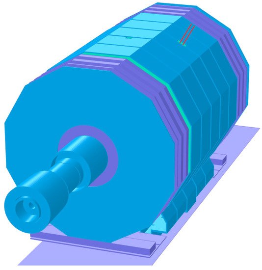
Figure 2. Three-dimensional model of the CMS magnet [54], using the TOSCA program for calculating the magnetic flux at a solenoid current of 18.164 kA. The ferromagnetic materials of the magnet yoke are marked with different color shades, in which three different magnetization curves are used. Shown are five steel barrel wheels, W0, W ± 1, and W ± 2, with their feet; four steel endcap disks, D ± 1, D ± 2, D ± 3, and D ± 4, on each side of the central part with the upper parts of their carts; the most distant ferromagnetic elements of the model, extending to distances of ±21.89 m in both directions from the centre of the solenoid; steel absorbers and collars of the forward hadron calorimeter; ferromagnetic elements of the radiation shielding; and collimators of the proton beams. Two linear conductors of the current leads in a special chimney in the W–1 barrel wheel, a chimney in the W + 1 barrel wheel for pipelines of the cryogenic system, and a 40 mm thick steel floor are seen as well.
According to the number of faces, the barrel wheels and endcap disks have 12 azimuthal sectors, 30° each. The sectors are numbered in the direction of increasing the values of the azimuthal angle and the numbering starts from a horizontally located sector S1, the middle of which coincides with the X axis. As can be seen from Figure 3a, each barrel wheel sector consists of three layers, connected by steel brackets, one (L1) of 0.285 m thick and two (L2 and L3) of 0.62 m thick each. Thick layers consist of two types of steel—steel G is in 0.085 m thick linings and steel I is in a core with a thickness of 0.45 m.
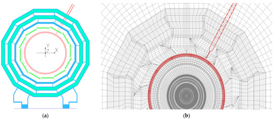
Figure 3. (a) Model of the central barrel wheel W0 with steel feet and a floor in the presence of four layers of superconducting cable and two linear current conductors and (b) finite element mesh in the XY plane.
The distance between the thin layer L1 and the middle thick layer L2 is 0.45 m, the same between two thick layers is 0.405 m. The air gaps between the central barrel wheel W0 and the adjacent wheels W ± 1 are 0.155 m each, the gaps between the wheels W ± 1 and W ± 2 are equal to 0.125 m each [51].
There is an additional fourth TC layer of 0.18 m thick in the central wheel W0 at 3.868 m from the solenoid axis, which absorbs hadrons escaping the barrel hadron calorimeter due to its insufficient thickness at low values of pseudorapidity. The blocks of this layer are displaced in the azimuth angle by 5° with respect to other blocks in the sector [52]. The distance between the layers TC and L1 is 0.567 m, and their material is steel G. The same type of steel is used in the connecting brackets and the barrel wheel feet. The material for the floor of the experimental underground cavern is steel S.
Steel S is used in the large and small endcap disks that close the flux-return yoke on each side of the solenoid cryostat, as well as in the connection rings between them and in the plates of the disk carts. The thickness of each of the first two disks is 0.592 m, the third disk is 0.232 m thick, and the fourth small disk is 0.075 m. The air gaps between the W ± 2 barrel wheels and the D ± 1 disks are 0.649 m each, the gaps between the D ± 1 and D ± 2 disks are 0.663 m each, the gaps between the D ± 2 and D ± 3 disks are 0.668 m each and, finally, the gaps between the D ± 3 and D ± 4 disks are 0.664 m each [51].
In 2013–2014 the fourth small disk of 5 m in diameter was increased to an inscribed diameter of 13.91 m, and the thickness of this outer part of the disk is 0.125 m [52]. The extended part of the fourth disk consists of two steel plates, each 25 mm thick, and a specialized concrete between them containing oxides of boron and iron, while the iron content is 57%. In the model the magnetization curve of steel G is used for the fourth disk’s extended plates, and concrete is described by the same curve with a packing factor of 0.57.
When building a three-dimensional model, a two-dimensional mesh of finite elements is created initially in the XY plane, as shown in Figure 3b, where all ferromagnetic elements used in the model are discretised. Then this mesh is extruded layer-by-layer in the direction of the Z axis, while the coordinates of the mesh nodes are transformed to describe complex geometric volumes, mainly cylindrical and conical, with a minimum number of the plane mesh nodes. Layers in the Z direction and the location of elements in the XY planes between them are used to describe the materials of the model elements. At present, the model of the CMS magnetic system contains 140 layers and 8,759,730 nodes of the spatial mesh in a cylindrical volume with a diameter of 100 m and a length of 120 m.
5. Magnetization Curves of Steel in the CMS Magnet Model
To describe the properties of the ferromagnetic elements of the CMS magnetic system, the model uses three curves of the isotropic nonlinear dependence of the magnetic flux density B on the magnetic field strength H [50], presented in Figure 4 on a semi-log scale.
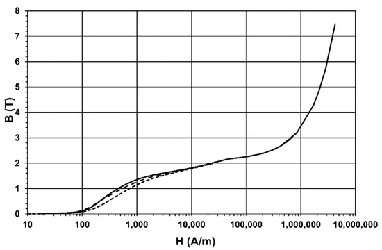
Figure 4. Magnetization curves of the steel used in the CMS magnet. Steel I (dashed line) is used to produce blocks of the barrel wheel thick layers. Steel S (dotted line) is used to produce the yoke nose and endcap disks. The same B–H curve in the model describes the magnetic properties of the disk carts and the floor of the experimental cavern. The magnetization curve of steel G (solid line) is used in the model for all other ferromagnetic elements.
Each B-H curve was obtained by averaging the magnetization curves measured for samples corresponding to different melts of a given type of steel used in the flux-return yoke elements. For the magnetization curve of steel G, averaging was performed over 33 samples, while scattering between the magnetization curves of the samples was, on average, (11.5 ± 9.1)%. For the magnetization curve of steel I, averaging was performed over 65 samples, and a spread between the magnetization curves of the samples was, on average, (8.7 ± 8.0)%. For the magnetization curve of steel S averaging was performed over 72 samples, while a dispersion between the magnetization curves of the samples was, on average, (8.2 ± 7.8)%.
The magnetization curves of steel samples were measured in the range B from 0.003 to 2 T. For the magnetic flux density values exceeding 2.15 T, all curves use the magnetization curve of steel I, measured up to a B value of 7.4887 T. In this interval, the dependence of B vs. H becomes linear with a slope coefficient greater than the magnetic permeability of vacuum by 0.42%.
This entry is adapted from the peer-reviewed paper 10.3390/sym13061052
References
- Klioukhine, V.; Campi, D.; Cure, B.; Desirelli, A.; Farinon, S.; Gerwig, H.; Grillet, J.; Herve, A.; Kircher, F.; Levesy, B.; et al. 3D magnetic analysis of the CMS magnet. IEEE Trans. Appl. Supercond. 2000, 10, 428–431.
- Klyukhin, V.I.; Ball, A.; Campi, D.; Cure, B.; Dattola, D.; Gaddi, A.; Gerwig, H.; Hervé, A.; Loveless, R.; Reithler, H.; et al. Measuring the Magnetic Field Inside the CMS Steel Yoke Elements. In Proceedings of the 2008 IEEE Nuclear Science Symposium Conference Record, Dresden, Germany, 19–25 October 2008; pp. 2270–2273.
- Klyukhin, V.I.; Amapane, N.; Andreev, V.; Ball, A.; Cure, B.; Herve, A.; Gaddi, A.; Gerwig, H.; Karimaki, V.; Loveless, R.; et al. The CMS Magnetic Field Map Performance. IEEE Trans. Appl. Supercond. 2010, 20, 152–155.
- Klyukhin, V.I.; Amapane, N.; Ball, A.; Cure, B.; Gaddi, A.; Gerwig, H.; Mulders, M.; Herve, A.; Loveless, R. Measuring the Magnetic Flux Density in the CMS Steel Yoke. J. Supercond. Nov. Magn. 2012, 26, 1307–1311.
- Klyukhin, V.I.; Amapane, N.; Ball, A.; Cure, B.; Gaddi, A.; Gerwig, H.; Mulders, M.; Calvelli, V.; Herve, A.; Loveless, R. Validation of the CMS Magnetic Field Map. J. Supercond. Nov. Magn. 2014, 28, 701–704.
- Klyukhin, V.I.; Amapane, N.; Ball, A.; Curé, B.; Gaddi, A.; Gerwig, H.; Mulders, M.; Hervé, A.; Loveless, R. Flux Loop Measurements of the Magnetic Flux Density in the CMS Magnet Yoke. J. Supercond. Nov. Magn. 2016, 30, 2977–2980.
- Klyukhin, V.I.; Cure, B.; Amapane, N.; Ball, A.; Gaddi, A.; Gerwig, H.; Herve, A.; Loveless, R.; Mulders, M. Using the Standard Linear Ramps of the CMS Superconducting Magnet for Measuring the Magnetic Flux Density in the Steel Flux-Return Yoke. IEEE Trans. Magn. 2018, 55, 8300504.
- TOSCA/OPERA-3d 18R2 Reference Manual; Cobham CTS Ltd.: Kidlington, UK, 2018; pp. 1–916.
- Simkin, J.; Trowbridge, C. Three-dimensional nonlinear electromagnetic field computations, using scalar potentials. In IEE Proceedings B Electric Power Applications; Institution of Engineering and Technology (IET): London, UK, 1980; Volume 127, pp. 368–374.
- Simkin, J.; Trowbridge, C.W. On the use of the total scalar potential on the numerical solution of fields problems in electromagnetics. Int. J. Numer. Methods Eng. 1979, 14, 423–440.
- Landau, L.D.; Lifshitz, E.M. Electrodynamics of Continuous Media, 2nd ed.; Nauka: Moscow, Russia, 1982; pp. 154–163. (In Russian)
- Tamm, I.E. Fundamentals of the Theory of Electricity, 9th ed.; Nauka: Moscow, Russia, 1976; pp. 285–288. (In Russian)
- Vishnyakov, I.A.; Vorob’ev, A.P.; Kechkin, V.F.; Klyukhin, V.I.; Kozlovsky, E.A.; Malyaev, V.K.; Selivanov, G.I. Superconducting solenoid for a colliding beams device. Sov. Phys. Tech. Phys. 1992, 37, 195–201.
- The DØ Collaboration. E823 (DØ Upgrade): Magnetic Tracking; D0 Note 1933; FNAL: Batavia, IL, USA, 1993. Available online: (accessed on 9 June 2021).
- The DØ Collaboration. DØ Upgrade. FERMILAB-PROPOSAL-0823; FNAL: Batavia, IL, USA, 1993. Available online: (accessed on 9 June 2021).
- The DØ Collaboration. The DØ Upgrade. FERMILAB-Conf-95/177-E; FNAL: Batavia, IL, USA, 1995. Available online: (accessed on 9 June 2021).
- Wayne, M.R. The DØ upgrade. Nucl. Instrum. Methods Phys. Res. Sect. A Accel. Spectrometer Detect. Assoc. Equip. 1998, 408, 103–109.
- CMS. The Magnet Project; Technical Design Report, CERN/LHCC 97-10, CMS TDR 1; CERN: Geneva, Switzerland, 1997; ISBN 92-9083-101-4. Available online: (accessed on 9 June 2021).
- ATLAS. Magnet System; Technical Design Report, CERN/LHCC 97-18, ATLAS TDR 6; CERN: Geneva, Switzerland, 1997; ISBN 92-9083-104-9. Available online: (accessed on 9 June 2021).
- Galić, H.; Wohl, C.; Armstrong, B.; Dodder, D.; Klyukhin, V.; Ryabov, Y.; Illarionova, N.; Lehar, F.; Oyanagi, Y.; Olin, A.; et al. Current Experiments in Elementary Particle Physics. Technical Report LBL-91-Rev.-6-92; 1992; p. 131. Available online: (accessed on 9 June 2021).
- Galic, H.; Lehar, F.; Klyukhin, V.; Ryabov, Y.; Bilak, S.; Illarionova, N.; Khachaturov, B.; Strokovsky, E.; Hoffman, C.; Kettle, P.-R.; et al. Current Experiments in Particle Physics. Technical Report LBL-91-Rev.-9-96; 1996; p. 46. Available online: (accessed on 9 June 2021).
- The LHC Study Group. Design Study of the Large Hadron Collider (LHC). A Multiparticle Collider in the LEP Tunnel; CERN-91-03, CERN-AC-DI-FA-90-06-REV; CERN: Geneva, Switzerland, 1991.
- CMS. The Compact Muon Solenoid. Letter of Intent by the CMS Collaboration for a General Purpose Detector at the LHC; CERN/LHCC/92-3; LHCC/I 1; CERN: Geneva, Switzerland, 1992; Available online: (accessed on 9 June 2021).
- ATLAS. Letter of Intent for a General-Purpose PP Experiment at the Large Hadron Collider at CERN; CERN/LHCC/92-4, LHCC/I 2; CERN: Geneva, Switzerland, 1992; Available online: (accessed on 9 June 2021).
- Erdogan, A.; Zmushko, V.V.; Klyukhin, V.I.; Froidevaux, D. Study of the H → WW → lνjj and H → ZZ → lljj decays for mH = 1 TeV/c2 at the LHC energies. Yadernaya Fizika 1994, 59, 290–301. (In Russian)
- Erdogan, A.; Froidevaux, D.; Klyukhin, V.; Zmushko, V. On the Experimental study of the H → WW → lνjj and H → ZZ → lljj Decays for mH = 1 TeV/c2 at LHC energies. Phys. Atom. Nucl. 1994, 57, 274–284.
- Zmushko, S.; Erdogan, A.; Froidevaux, D.; Klioukhine, S. Study of H → WW → Lνjj and H → ZZ → Lljj Decays for mH = 1 TeV; ATLAS Internal note PHYS-No-008; CERN: Geneva, Switzerland, 1992; Available online: (accessed on 9 June 2021).
- ATLAS. Technical Proposal for a General-Purpose PP Experiment at the Large Hadron Collider at CERN; CERN/LHCC/94-43, LHCC/P2; CERN: Geneva, Switzerland, 1994; pp. 233–235. ISBN 92-9083-067-0. Available online: (accessed on 9 June 2021).
- Klyukhin, V.I.; Poppleton, A.; Schmitz, J. Magnetic Field Integrals for the ATLAS Tracking Volume; IHEP: Protvino, Russia, 1993.
- Klyukhin, V.I.; Poppleton, A.; Schmitz, J. Field Integrals for the ATLAS Tracking Volume; ATLAS Internal note INDET-NO-023; CERN: Geneva, Switzerland, 1993; Available online: (accessed on 9 June 2021).
- ALICE. Technical Proposal for a Large Ion Collider Experiment at the LHC; CERN/LHCC 95-71, LHCC/P3; CERN: Geneva, Switzerland, 1995; pp. 99–101. ISBN 92-9083-088-077-8. Available online: (accessed on 9 June 2021).
- ALICE. The Forward Muon Spectrometer; Addendum to the ALICE Technical Proposal. CERN/LHCC 96-32, LHCC/P3-Addendum 1; CERN: Geneva, Switzerland, 1996; pp. 9–10. ISBN 92-9083-088-3. Available online: (accessed on 9 June 2021).
- Herve, A. Constructing a 4-Tesla Large Thin Solenoid at the Limit of What Can Be Safely Operated. Mod. Phys. Lett. A 2010, 25, 1647–1666.
- Kircher, F.; Bredy, P.; Calvo, A.; Cure, B.; Campi, D.; Desirelli, A.; Fabbricatore, P.; Farinon, S.; Herve, A.; Horvath, I.; et al. Final design of the CMS solenoid cold mass. IEEE Trans. Appl. Supercond. 2000, 10, 407–410.
- Herve, A.; Blau, B.; Bredy, P.; Campi, D.; Cannarsa, P.; Cure, B.; Dupont, T.; Fabbricatore, P.; Farinon, S.; Feyzi, F.; et al. Status of the Construction of the CMS Magnet. IEEE Trans. Appl. Supercond. 2004, 14, 542–547.
- Campi, D.; Cure, B.; Gaddi, A.; Gerwig, H.; Herve, A.; Klyukhin, V.; Maire, G.; Perinic, G.; Bredy, P.; Fazilleau, P.; et al. Commissioning of the CMS Magnet. IEEE Trans. Appl. Supercond. 2007, 17, 1185–1190.
- CMS Collaboration. Commissioning and performance of the CMS pixel tracker with cosmic ray muons. J. Instrum. 2010, 5, T03007.
- CMS Collaboration. Commissioning and performance of the CMS silicon strip tracker with cosmic ray muons. J. Instrum. 2010, 5, T03008.
- CMS Collaboration. Performance and operation of the CMS electromagnetic calorimeter. J. Instrum. 2010, 5, T03010.
- CMS Collaboration. Performance of the CMS hadron calorimeter with cosmic ray muons and LHC beam data. J. Instrum. 2010, 5, T03012.
- CMS Collaboration. Performance of the CMS drift tube chambers with cosmic rays. J. Instrum. 2010, 5, T03015.
- CMS Collaboration. Performance of the CMS cathode strip chambers with cosmic rays. J. Instrum. 2010, 5, T03018.
- CMS Collaboration. Performance study of the CMS barrel resistive plate chambers with cosmic rays. J. Instrum. 2010, 5, T03017.
- CMS Collaboration. Performance of CMS muon reconstruction in cosmic-ray events. J. Instrum. 2010, 5, T03022.
- Abdullin, S.; The CMS-HCAL Collaboration; Abramov, V.; Acharya, B.; Adams, M.; Akchurin, N.; Akgun, U.; Anderson, E.; Antchev, G.; Arcidy, M.; et al. Design, performance, and calibration of CMS forward calorimeter wedges. Eur. Phys. J. C 2007, 53, 139–166.
- CMS Collaboration. Precise mapping of the magnetic field in the CMS barrel yoke using cosmic rays. J. Instrum. 2010, 5, T03021.
- Herve, A. The CMS detector magnet. IEEE Trans. Appl. Supercond. 2000, 10, 389–394.
- Horvath, I.; Dardel, B.; Marti, H.-P.; Neuenschwander, J.; Smith, R.; Fabbricatore, P.; Musenich, R.; Calvo, A.; Campi, D.; Cure, B.; et al. The CMS conductor. IEEE Trans. Appl. Supercond. 2000, 10, 395–398.
- Klyukhin, V.I.; Ball, A.; Campi, D.; Cure, B.; Dattola, D.; Gaddi, A.; Gerwig, H.; Hervé, A.; Loveless, R.; Reithler, H.; et al. Measuring the Magnetic Field Inside the CMS Steel Yoke Elements. In Proceedings of the 2008 IEEE Nuclear Science Symposium Conference Record, Dresden, Germany, 19–25 October 2008; pp. 2270–2273.
- Klyukhin, V.I.; Amapane, N.; Andreev, V.; Ball, A.; Cure, B.; Herve, A.; Gaddi, A.; Gerwig, H.; Karimaki, V.; Loveless, R.; et al. The CMS Magnetic Field Map Performance. IEEE Trans. Appl. Supercond. 2010, 20, 152–155.
- Klyukhin, V.I.; Amapane, N.; Ball, A.; Cure, B.; Gaddi, A.; Gerwig, H.; Mulders, M.; Herve, A.; Loveless, R. Measuring the Magnetic Flux Density in the CMS Steel Yoke. J. Supercond. Nov. Magn. 2012, 26, 1307–1311.
- Klyukhin, V.I.; Amapane, N.; Ball, A.; Cure, B.; Gaddi, A.; Gerwig, H.; Mulders, M.; Calvelli, V.; Herve, A.; Loveless, R. Validation of the CMS Magnetic Field Map. J. Supercond. Nov. Magn. 2014, 28, 701–704.
- Klyukhin, V.I.; Amapane, N.; Ball, A.; Curé, B.; Gaddi, A.; Gerwig, H.; Mulders, M.; Hervé, A.; Loveless, R. Flux Loop Measurements of the Magnetic Flux Density in the CMS Magnet Yoke. J. Supercond. Nov. Magn. 2016, 30, 2977–2980.
- Klyukhin, V.I.; Cure, B.; Amapane, N.; Ball, A.; Gaddi, A.; Gerwig, H.; Herve, A.; Loveless, R.; Mulders, M. Using the Standard Linear Ramps of the CMS Superconducting Magnet for Measuring the Magnetic Flux Density in the Steel Flux-Return Yoke. IEEE Trans. Magn. 2018, 55, 8300504.
This entry is offline, you can click here to edit this entry!