In the learning paradigms of artificial neural networks, classical algorithms such as back-propagation aim to approach the theories of biological learning through an iterative adjustment of all the hyper-parameters of the hidden layers for each sequence of data. Therefore, without looking at relearning, in actual problems, the tuning process could take days or months under the use of the available ordinary computers for generalization of the neural network over all of the selected samples. But, the fact that a microprocessor is faster than a brain by about twelve million times, denies that these algorithms are capable of responding to the thought of the human brain which takes less seconds to classify or restore new images or sensations.
In 2004, ELM gave birth to new learning rules for artificial neural networks. ELM learning rules remove barriers between human biological thought and artificial neural networks by addressing the fact that: "the parameters of the hidden layer do not need to be adjusted, and the only element responsible for the "universal approximation and generalization are the output weights ". Consequently, ELM has been studied through several applications and extends to a multitude of paradigms such as the ensemble, the hybrid and the deep learning and achieved an excellent reputation. Therefore, The aim of this review will be introducing basic theories of ELM.
- Extreme Learning Machine
- ELM
- Single hidden layer feedforward neural network
ELM was first proposed for training a feedforward neural network with a single hidden layer[1]. Then, it expands to adapt to a variety of architectures to meet several types of applications and learning paradigms. The ELM basic learning rules were obtained based on the least squares method which uses the “Moore-Penrose” the pseudo-inverse of the matrix for the adjustment of the hyper-parameters.
Unlike old complex algorithms such as backpropagation, contrastive divergence, Swarm intelligence and Lagrange optimization, the first given rules of the ELM algorithm describe an of offline learning which can be simplified only in three steps.
For a given training set S = {X, T} such that X and T are its inputs and outputs respectively, the learning of ELM steps are:
- Step 01: The matrix of the input weights a and the vector of the bias b are generated randomly from any available stochastic distribution, separately from the training data.
- Step 02: The hidden layer H of the dataset is mapped and activated using any continuous limited activation function G as indicated in equation 1.

- Step 03: the output weights must be determined analytically using the pseudo-inverse of the hidden layer as explained by equation 2.

ELM rules attempt to solve the minimization problem presented in equation 3.

The Figure below shows the architecture of ELM networks with its basic parameters notations.
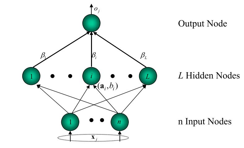
The number of hidden nodes in ELM is determined experimentally according to each type of application. Generally, the more hidden nodes, the more precision can be achieved.
The ELM algorithm has no settings for the learning rate or tolerance functions, which simplifies learning paradigms and reduces human intervention. In addition to this, the ELM algorithms have been tested on small capacity personal computers and prove that it does not need expensive computing resources [3].
References
- G. Bin Huang, Q. Y. Zhu, and C. K. Siew, “Extreme learning machine: A new learning scheme of feedforward neural networks,” IEEE Int. Conf. Neural Networks - Conf. Proc., vol. 2, no. August, pp. 985–990, 2004.
- G. Bin Huang, “What are Extreme Learning Machines? Filling the Gap Between Frank Rosenblatt’s Dream and John von Neumann’s Puzzle,” Cognit. Comput., vol. 7, no. 3, pp. 263–278, 2015.
- G. Huang, “An Insight into Extreme Learning Machines : Random Neurons , Random Features and Kernels,” Springer New York LLC, vol. 6, no. 3, pp. 376–390, 2014