With the significant advancement of sensor and communication technology and the reliable application of obstacle detection techniques and algorithms, automated driving is becoming a pivotal technology that can revolutionize the future of transportation and mobility. Sensors are fundamental to the perception of vehicle surroundings in an automated driving system, and the use and performance of multiple integrated sensors can directly determine the safety and feasibility of automated driving vehicles.
- autonomous vehicles
- self-driving cars
- perception
- camera
- lidar
- radar
- sensor fusion
- calibration
- obstacle detection
1. Introduction
According to the Global Status Report published by the World Health Organization (WHO), the reported number of annual road traffic deaths reached 1.35 million in 2018, making it the world’s eighth leading cause of unnatural death among people of all ages [1]. In the context of the European Union (EU), while there has been a decrease in the reported annual road fatalities, there is still more than 40,000 fatalities per annum, 90% of which were caused by human error. For this reason and to improve traffic flows, global investors have invested significantly to support the development of self-driving vehicles. Additionally, it is expected that the autonomous vehicles (AVs) will help to reduce the level of carbon emissions, and hence contribute to carbon emissions reduction targets [2].
AVs or self-driving vehicles provide the transportation capabilities of conventional vehicles but are largely capable of perceiving the environment and self-navigating with minimal or no human intervention. According to a report published by the Precedence Research, the global AV market size reached approximately 6500 units in 2019 and is predicted to experience a compound annual growth rate of 63.5% over the period 2020 to 2027 [3]. In 2009, Google secretly initiated its self-driving car project, currently known as Waymo (and presently a subsidiary of Google parent company Alphabet). In 2014, Waymo revealed a 100% autonomous car prototype without pedals and steering wheel [4]. To date, Waymo has achieved a significant milestone, whereby its AVs had collectively driven over 20 million miles on public roads in 25 cities in the United States of America (USA) [5]. Within the Irish context, in 2020, Jaguar Land Rover (JLR) Ireland has announced its collaboration with autonomous car hub in Shannon, Ireland, and will use 450 km of roads to test its next-generation AV technology [6].
In 2014, the SAE International, previously known as the Society of Automotive Engineers (SAE) introduced the J3016 “Levels of Driving Automation” standard for consumers. The J3016 standard defines the six distinct levels of driving automation, starting from SAE level 0 where the driver is in full control of the vehicle, to SAE level 5 where vehicles can control all aspects of the dynamic driving tasks without human intervention. The overview of these levels is depicted in Figure 1 and are often cited and referred to by industry in the safe design, development, testing, and deployment of highly automated vehicles (HAVs) [7]. Presently, automobile manufacturers such as Audi (Volkswagen) and Tesla adopted the SAE level 2 automation standards in developing its automation features, namely Tesla’s Autopilot [8] and Audi A8′s Traffic Jam Pilot [9,10]. Alphabet’s Waymo, on the other hand, has since 2016 evaluated a business model based on SAE level 4 self-driving taxi services that could generate fares within a limited area in Arizona, USA [11].
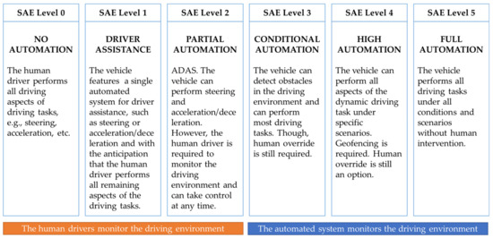
Figure 1. An overview of the six distinct levels of driving automation that were described in the Society of Automotive Engineers (SAE) J3016 standard. Readers interested in the comprehensive descriptions of each level are advised to refer to SAE International. Figure redrawn and modified based on depictions in [7].
Most autonomous driving (AD) systems share many common challenges and limitations in real-world situations, e.g., safe driving and navigating in harsh weather conditions, and safe interactions with pedestrians and other vehicles. Harsh weather conditions, such as glare, snow, mist, rain, haze, and fog, can significantly impact the performance of the perception-based sensors for perception and navigation. Besides, the challenges for AD in adverse weather are faced in other constrained AD scenarios like agriculture and logistics. For on-road AVs, the complexity of these challenges increases because of the unexpected conditions and behaviors from other vehicles. For example, placing a yield sign in an intersection can change the behavior of the approaching vehicles. Hence, a comprehensive prediction module in AVs is critical to identify all position future motions to reduce collision hazards [12,13]. Although AD systems share many common challenges in real-world situations, they are differed noticeably in several aspects. For instance, unmanned tractors in agriculture farm navigates between crop rows in a fixed environment, while on-road vehicles must navigate through complex dynamic environment, such as crowds and traffics [14].
2. Sensor Technology in Autonomous Vehicles
Sensors are devices that map the detected events or changes in the surroundings to a quantitative measurement for further processing. In general, sensors are classified into two classes based on their operational principal. Proprioceptive sensors, or internal state sensors, capture the dynamical state and measures the internal values of a dynamic system, e.g., force, angular rate, wheel load, battery voltage, et cetera. Examples of the proprioceptive sensors include Inertia Measurement Units (IMU), encoders, inertial sensors (gyroscopes and magnetometers), and positioning sensors (Global Navigation Satellite System (GNSS) receivers). In contrast, the exteroceptive sensors, or external state sensors, sense and acquire information such as distance measurements or light intensity from the surroundings of the system. Cameras, Radio Detection and Ranging (Radar), Light Detection and Ranging (LiDAR), and ultrasonic sensors are examples of the exteroceptive sensors. Additionally, sensors can either be passive sensors or active sensors. Passive sensors receive energy emitting from the surroundings to produce outputs, e.g., vision cameras. Conversely, active sensors emit energy into the environment and measure the environmental “reaction” to that energy to produce outputs, such as with LiDAR and radar sensors [27,28,29].
In AVs, sensors are critical to the perception of the surroundings and localization of the vehicles for path planning and decision making, essential precursors for controlling the motion of the vehicle. AV primarily utilizes multiple vision cameras, radar sensors, LiDAR sensors, and ultrasonic sensors to perceive its environment. Additionally, other sensors, including the Global Navigation Satellite System (GNSS), IMU, and vehicle odometry sensors are used to determine the relative and absolute positions of the vehicle [30]. The relative localization of an AV refers to the vehicles referencing of its coordinates in relation to the surrounding landmarks, while absolute localization refers to the vehicle referencing its position in relation to a global reference frame (world) [31]. The placement of sensors for environment perception on typical AV applications, their coverage, and applications are shown in Figure 3. The reader will appreciate that in a moving vehicle, there is a more complete coverage of the vehicle’s surroundings. The individual and relative positioning of multiple sensors are critical for precise and accurate object detection and therefore reliably and safely performing any subsequent actions [32]. In general, it is challenging to generate adequate information from a single independent source in AD. This section reviews the advantages and shortcomings of the three primary sensors: cameras, LiDARs and radars, for environment perception in AV applications.
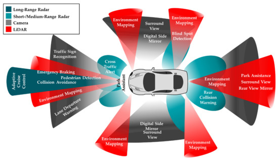
Figure 3. An example of the type and positioning of sensors in an automated vehicle to enable the vehicles perception of its surrounding. Red areas indicate the LiDAR coverage, grey areas show the camera coverage around the vehicle, blue areas display the coverage of short-range and medium-range radars, and green areas indicate the coverage of long-range radar, along with the applications the sensors enable—as depicted in [32] (redrawn).
2.1. Camera
Cameras are one of the most adopted technology for perceiving the surroundings. A camera works on the principle of detecting lights emitted from the surroundings on a photosensitive surface (image plane) through a camera lens (mounted in front of the sensor) to produce clear images of the surrounding [20,30]. Cameras are relatively inexpensive and with appropriate software, can detect both moving and static obstacles within their field of view and provides high-resolution images of the surroundings. These capabilities allow the perception system of the vehicle to identify road signs, traffic lights, road lane markings and barriers in the case of road traffic vehicles and a host of other articles in the case of off-road vehicles. The camera system in an AV may employ monocular cameras or binocular cameras, or a combination of both. As the name implies, the monocular camera system utilizes a single camera to create a series of images. The conventional RGB monocular cameras are fundamentally more limited than stereo cameras in that they lack native depth information, although in some applications or more advanced monocular cameras using the dual-pixel autofocus hardware, depth information may be calculated using complex algorithms [33,34,35]. As a result, two cameras are often installed side-by-side to form a binocular came-ra system in autonomous vehicles.
The stereo camera, also known as a binocular camera, imitates the perception of depth found in animals, whereby the “disparity” between the slightly different images formed in each eye is (subconsciously) employed to provide a sense of depth. Stereo cameras contain two image sensors, separated by a baseline. The term baseline refers to the distance between the two image sensors (and is generally cited in the specifications of stereo cameras), and it differs depending on the camera’s model. For example, the Orbbec 3D cameras reviewed in [36] for Autonomous Intelligent Vehicles (AIV) has a baseline of 75 mm for both the Persee and Astra series cameras [37]. As in the case of animal vision, the disparity maps calculated from the stereo camera imagery permit the generation of depth maps using epipolar geometry and triangulation methods (detailed discussion of the disparity calculations algorithms is beyond the scope of this paper). Reference [38] uses the “stereo_image_proc” modules in Robotic Operating System (ROS), an open source, meta-operating system for robotics [39], to perform stereo vision processing before implementing SLAM (simultaneous localization and mapping) and autonomous navigation. Table 2 shows the general specifications for binocular cameras from different manufacturers.
Table 2. General specifications of stereo cameras from various manufacturers that we reviewed from our initial findings. The acronyms from left to right (in second row) are horizontal field-of-view (HFOV); vertical field-of-view (VFOV); frames per second (FPS); image resolutions in megapixels (Img Res); depth resolutions (Res); depth frames per second (FPS); and reference (Ref). The “-” symbol in table below indicates that the specifications were not mentioned in product datasheet.
| Depth Information | |||||||||||
|---|---|---|---|---|---|---|---|---|---|---|---|
| Model | Baseline (mm) | HFOV (°) | VFOV (°) | FPS (Hz) | Range (m) | Img Res (MP) | Range (m) | Res (MP) | FPS (Hz) | Ref | |
| Roboception | RC Visard 160 | 160 | 61 * | 48 * | 25 | 0.5–3 | 1.2 | 0.5–3 | 0.03–1.2 | 0.8–25 | [40,41] |
| Carnegie Robotics® | MultiSense™ S7 1 | 70 | 80 | 49/80 | 30 max | - | 2/4 | 0.4 min | 0.5–2 | 7.5–30 | [40,42,43] |
| MultiSense™ S21B 1 | 210 | 68–115 | 40–68 | 30 max | - | 2/4 | 0.4 min | 0.5–2 | 7.5–30 | [40,44] | |
| Ensenso | N35-606-16-BL | 100 | 58 | 52 | 10 | 4 max | 1.3 | - | [40,45] | ||
| Framos | D435e | 55 | 86 | 57 | 30 | 0.2–10 | 2 | 0.2 min | 0.9 | 30 | [40,46] |
| Nerian | Karmin3 2 | 50/100/250 | 82 | 67 | 7 | - | 3 | 0.23/0.45/1.14 min | 2.7 | - | [40,47] |
| Intel RealSense | D455 | 95 | 86 | 57 | 30 | 20 max | 3 | 0.4 min | ≤1 | ≤90 | [40,48] |
| D435 | 50 | 86 | 57 | 30 | 10 max | 3 | 0.105 min | ≤1 | ≤90 | ||
| D415 | 55 | 65 | 40 | 30 | 10 max | 3 | 0.16 min | ≤1 | ≤90 | ||
| Flir® | Bumblebee2 3 | 120 | 66 | - | 48/20 | - | 0.3/0.8 | - | [40,49] | ||
| Bumblebee XB3 3 | 240 | 66 | - | 16 | - | 1.2 | [50,51] | ||||
Other commonly employed cameras in AVs for perception of the surroundings include fisheye cameras [52,53,54]. Fisheye cameras are commonly employed in near-field sensing applications, such as parking and traffic jam assistance, and require only four cameras to provide a 360-degree view of the surroundings. Reference [52] proposed a fisheye surround-view system and the convolutional neural network (CNN) architecture for moving object segmentation in an autonomous driving environment, running at 15 frames per second at an accuracy of 40% Intersection over Union (IoU, in approximate terms, an evaluation metric that calculates the area of overlap between the target mask (ground truth) and predicted mask), and 69.5% mean IoU.
The deviation in lens geometry from the ideal/nominal geometry will result in image distortion, such that in extreme cases, e.g., ultra-wide lenses employed in fisheye cameras, straight lines in the physical scene may become curvilinear. In photography, the deviations in camera lens geometry are generally referred to as optical distortion, and are commonly categorized as pincushion distortion, barrel distortion, and moustache distortion. Such distortions may introduce an error in the estimated location of the detected obstacles or features in the image. Hence, it is often a require to “intrinsically calibrate” the camera to estimate the camera parameters and rectify the geometric distortions [55]. We present a detailed discussion of the camera intrinsic calibration and the commonly employed method in Section 3.1.1. Further, it is known that the quality (resolution) of images captured by the cameras may significantly affected by lighting and adverse weather conditions, e.g., snow, intense sun glare, rainstorm, hazy weather, et cetera. Other disadvantages of cameras may include the requirement for large computation power while analyzing the image data [20].
Given the above, cameras are a ubiquitous technology that provides high-resolution videos and images, including color and texture information of the perceived surroundings. Common uses of the camera data on AVs include traffic signs recognition, traffic lights recognition, and road lane marking detection. As the camera’s performance and the creation of high-fidelity images are highly dependent on the environmental conditions and illumination, image data are often fused with other sensor data such as radar and LiDAR data, to generate reliable and accurate environment perception in AD.
2.2. LiDAR
Light Detection and Ranging, or LiDAR, was first established in the 1960s and was widely used in the mapping of aeronautical and aerospace terrain. In the mid-1990s, laser scanners manufacturers produced and delivered the first commercial LiDARs with 2000 to 25,000 pulses per second (PPS) for topographic mapping applications [56]. The development of LiDAR technologies has evolved continuously at a significant pace over the past few decades and is currently one of the cores perception technologies for Advanced Driver Assistance System (ADAS) and AD vehicles. LiDAR is a remote sensing technology that operates on principle of emitting pulses of infrared beams or laser light which reflect off target objects. These reflections are detected by the instrument and the interval taken between emission and receiving of the light pulse enables the estimation of distance. As the LiDAR scans its surroundings, it generates a 3D representation of the scene in the form of a point cloud [20].
The rapid growth of research and commercial enterprises relating to autonomous robots, drones, humanoid robots, and AVs has established a high demand for LiDAR sensors due to its performance attributes such as measurement range and accuracy, robustness to surrounding changes and high scanning speed (or refresh rate)—for example, typical instruments in use today may register up to 200,000 points per second or more, covering 360° rotation and a vertical field of view of 30°. As a result, many LiDAR sensor companies have emerged and have been introducing new technologies to address these demands in recent years. Hence, the revenue of the automotive LiDAR market is forecasted to reach a total of 6910 million USD by 2025 [57]. The wavelengths of the current state-of-the-art LiDAR sensors exploited in AVs are commonly 905 nm (nanometers)—safest types of lasers (Class 1), which suffers lower absorption water than for example 1550 nm wavelength sensors which were previously employed [58]. A study in reference [59] found that the 905 nm systems can provide higher resolution of point clouds in adverse weather conditions like fog and rains. The 905 nm LiDAR systems, however, are still partly sensitive to fog and precipitation: a recent study in [60] conveyed that harsh weather conditions like fogs and snows could degrade the performance of the sensor by 25%.
The three primary variants of LiDAR sensors that can be applied in a wide range of applications include 1D, 2D and 3D LiDAR. LiDAR sensors output data as a series of points, also known as point cloud data (PCD) in either 1D, 2D and 3D spaces and the intensity information of the objects. For 3D LiDAR sensors, the PCD contains the x, y, z coordinates and the intensity information of the obstacles within the scene or surroundings. For AD applications, LiDAR sensors with 64- or 128- channels are commonly employed to generate laser images (or point cloud data) in high resolution [61,62].
-
1D or one-dimensional sensors measure only the distance information (x-coordinates) of objects in the surroundings.
-
2D or two-dimensional sensors provides additional information about the angle (y-coordinates) of the targeted objects.
-
3D or three-dimensional sensors fire laser beams across the vertical axes to measure the elevation (z-coordinates) of objects around the surroundings.
LiDAR sensors can further be categorized as mechanical LiDAR or solid-state LiDAR (SSL). The mechanical LiDAR is the most popular long-range environment scanning solution in the field of AV research and development. It uses the high-grade optics and rotary lenses driven by an electric motor to direct the laser beams and capture the desired field of view (FoV) around the AV. The rotating lenses can achieve a 360° horizontal FoV covering the vehicle surroundings. Contrarily, the SSLs eliminate the use of rotating lenses and thus avoiding mechanical failure. SSLs use a multiplicity of micro-structured waveguides to direct the laser beams to perceive the surroundings. These LiDARs have gained interest in recent years as an alternative to the spinning LiDARs due to their robustness, reliability, and generally lower costs than the mechanical counterparts. However, they have a smaller and limited horizontal FoV, typically 120° or less, than the traditional mechanical LiDARs [30,63].
Reference [64] compares and analyzes 12 spinning LiDAR sensors that are currently available in the market from various LiDAR manufacturers. In [64], different models and laser configurations are evaluated in three different scenarios and environments, including dynamic traffic, adverse weather generated in a weather simulation chamber, and static targets. The results demonstrated that the Ouster OS1-16 LiDAR model had the lowest average number of points on reflective targets and the performance of spinning LiDARs are strongly affected by intense illumination and adverse weather, notable where precipitation is high and there is non-uniform or heavy fog. Table 3 shows the general specifications of each tested LiDAR sensor in the study of [64] (comprehensive device specifications are presented as well in [65]). In addition, we extended the summarized general specifications in the study of [64,65] with other LiDARs, including Hokuyo 210° spinning LiDAR and SSLs from Cepton, SICK, and IBEO, and the commonly used ROS drivers for data acquisition from our initial findings.
Laser returns are discrete observations that are recorded when a laser pulse is intercepted and reflected by the targets. LiDARs can collect multiple returns from the same laser pulse and modern sensors can record up to five returns from each laser pulse. For instance, the Velodyne VLP-32C LiDAR analyze multiple returns and reports either the strongest, last, or dual return, depending on the laser return mode configurations. In single laser return mode (strongest return or last return), the sensor analyzes lights received from the laser beam in one direction to determine the distance and intensity information and subsequently employs this information to determine the last return or strongest return. In contrast, sensors in dual return configuration mode will return both the strongest and last return measurements. However, the second-strongest measurements will return as the strongest if the strongest return measurements are like the last return measurements. Not to mention that points with insufficient intensity will be disregarded [66].
In general, at present, 3D spinning LiDARs are more commonly applied in self-driving vehicles to provide a reliable and precise perception of in day and night due to its broader field of view, farther detection range and depth perception. The acquired data in point cloud format provides a dense 3D spatial representation (or “laser image”) of the AVs’ surroundings. LiDAR sensors do not provide color information of the surroundings compared to the camera systems and this is one reason that the PCD is often fused with data from different sensors using sensor fusion algorithms.
Table 3. General specifications of the tested LiDARs from [64,65] and other LiDARs that were reviewed in the current work. The acronyms from left to right (first row) are frames per second (FPS); accuracy (Acc.); detection range (RNG); vertical FoV (VFOV); horizontal FoV (HFOV); horizontal resolution (HR); vertical resolution (VR); wavelength (λ); diameter (Ø); sensor drivers for Robotic Operating System (ROS Drv.); and reference for further information (Ref.). The “-” symbol in table below indicates that the specifications were not mentioned in product datasheet.
| Company | Model | Channels or Layers | FPS (Hz) | Acc. (m) | RNG (m) | VFOV (°) | HFOV (°) | HR (°) |
VR (°) |
λ (nm) | Ø (mm) | ROS Drv. | Ref. | |
|---|---|---|---|---|---|---|---|---|---|---|---|---|---|---|
| Mechanical/Spinning LiDARs | Velodyne | VLP-16 | 16 | 5–20 | ±0.03 | 1…100 | 30 | 360 | 0.1–0.4 | 2 | 903 | 103.3 | [67] | [51,68,69,70] |
| VLP-32C | 32 | 5–20 | ±0.03 | 1…200 | 40 | 360 | 0.1–0.4 | 0.33 1 | 903 | 103 | ||||
| HDL-32E | 32 | 5–20 | ±0.02 | 2…100 | 41.33 | 360 | 0.08–0.33 | 1.33 | 903 | 85.3 | ||||
| HDL-64E | 64 | 5–20 | ±0.02 | 3…120 | 26.8 | 360 | 0.09 | 0.33 | 903 | 223.5 | ||||
| VLS-128 Alpha Prime | 128 | 5–20 | ±0.03 | max 245 | 40 | 360 | 0.1–0.4 | 0.11 1 | 903 | 165.5 | - | |||
| Hesai | Pandar64 | 64 | 10,20 | ±0.02 | 0.3…200 | 40 | 360 | 0.2,0.4 | 0.167 1 | 905 | 116 | [71] | [72] | |
| Pandar40P | 40 | 10,20 | ±0.02 | 0.3…200 | 40 | 360 | 0.2,0.4 | 0.167 1 | 905 | 116 | [73] | |||
| Ouster | OS1–64 Gen 1 | 64 | 10,20 | ±0.03 | 0.8…120 | 33.2 | 360 | 0.7,0.35, 0.17 |
0.53 | 850 | 85 | [74] | [75,76] | |
| OS1-16 Gen 1 | 16 | 10,20 | ±0.03 | 0.8…120 | 33.2 | 360 | 0.53 | 850 | 85 | |||||
| RoboSense | RS-Lidar32 | 32 | 5,10,20 | ±0.03 | 0.4…200 | 40 | 360 | 0.1–0.4 | 0.33 1 | 905 | 114 | [77] | [78] | |
| LeiShen | C32-151A | 32 | 5,10,20 | ±0.02 | 0.5…70 | 32 | 360 | 0.09, 0.18,0.36 | 1 | 905 | 120 | [79] | [80] | |
| C16-700B | 16 | 5,10,20 | ±0.02 | 0.5…150 | 30 | 360 | 2 | 905 | 102 | [81] | [82] | |||
| Hokuyo | YVT-35LX-F0 | - | 20 3 | ±0.05 3 | 0.3…35 3 | 40 | 210 | - | - | 905 | ◊ | [83] | [84] | |
| Solid State LiDARs | IBEO | LUX 4L Standard | 4 | 25 | 0.1 | 50 2 | 3.2 | 110 | 0.25 | 0.8 | 905 | ◊ | [85] | [86] |
| LUX HD | 4 | 25 | 0.1 | 50 2 | 3.2 | 110 | 0.25 | 0.8 | 905 | ◊ | [87] | |||
| LUX 8L | 8 | 25 | 0.1 | 30 2 | 6.4 | 110 | 0.25 | 0.8 | 905 | ◊ | [88] | |||
| SICK | LD-MRS400102S01 HD | 4 | 50 | - | 30 2 | 3.2 | 110 | 0.125…0.5 | - | ◊ | [85] | [89] | ||
| LD-MRS800001S01 | 8 | 50 | - | 50 2 | 6.4 | 110 | 0.125…0.5 | - | ◊ | [90] | ||||
| Cepton | Vista P60 | - | 10 | - | 200 | 22 | 60 | 0.25 | 0.25 | 905 | ◊ | [91] | [92] | |
| Vista P90 | - | 10 | - | 200 | 27 | 90 | 0.25 | 0.25 | 905 | ◊ | [93] | |||
| Vista X90 | - | 40 | - | 200 | 25 | 90 | 0.13 | 0.13 | 905 | ◊ | [94] | |||
This entry is adapted from the peer-reviewed paper 10.3390/s21062140