Your browser does not fully support modern features. Please upgrade for a smoother experience.
Please note this is an old version of this entry, which may differ significantly from the current revision.
Subjects:
Engineering, Electrical & Electronic
In the energy-planning sector, the precise prediction of electrical load is a critical matter for the functional operation of power systems and the efficient management of markets.
- electrical load
- recurrent neural network
- short-term forecasting
1. Introduction
Electric load forecasting (ELF) in a power system is crucial for the operation planning of the system, and it also generates an increasing academic interest [1]. For the management and planning of the power system, forecasting demand factors such as load per hour, maximum (peak) load, and the total amount of energy is crucial. As a result, forecasting according to the time horizon is beneficial for meeting the various needs according to their application, as indicated in Table 1. The ELF is divided into three groups [2]:
Table 1. Applications of the forecasting processes based on time horizons.
| Time Horizon | Area of Application |
|---|---|
| 12 months–20 months | Planning of the Power System |
| 1 week–12 months | Scheduling the maintenance of the power system elements |
| 1 min–1 week | Commitment analysis of the power units |
| Automatic Generation Control (AGC) | |
| Economic load dispatch (ELD) | |
| ms–s | Power system dynamic analysis |
| ns–ms | Power system transient analysis |
-
Long-term forecasting (LTF): 1–20 years. The LTF is crucial for the inclusion of new-generation units in the system and the development of the transmission system.
-
Medium-term forecasting (MTF): 1 week–12 months. The MTF is most helpful for the setting of tariffs, the planning of the system maintenance, financial planning, and the scheduling of fuel supply.
-
Short-term forecasting (STF): 1 h–1 week. The STF is necessary for the data supply to the generation units to schedule their start-up and shutdown time, to prepare the spinning reserves, and to conduct an in-depth analysis of the restrictions in the transmission system. STF is also crucial for the evaluation of power system security.
Various approaches can be used based on the model found. Although MTF and LTF forecasting will rely on techniques such as trend analysis [3,4], end-use analysis [5], neural network technique [6,7,8,9,10], and multiple linear regressions [11], STF requires an approach based on regression [12], analysis of time series [13], implementation of artificial neural networks [14,15,16], expert systems [17], fuzzy logic [18,19], and support vector machines [20,21]. STF is important for both the Transmission System Operators (TSOs) in the case of extreme weather conditions to maintain the reliable operation of the system [22,23] and for the Distribution System Operators (DSOs) due to the constant increase of microgrids affecting the total load [24,25] as well as the difficulty of matching varying renewable energy to the demand with diminishing margins.
The MTF and LTF require both expertise in data analysis and experience of how power systems and the liberated markets function, but the STF relies more on data modeling (trying to fit data into models) than on in-depth knowledge of how a power system operates [26]. The load forecast of the day ahead (STF) is a work that the operational planning department of every TSO must establish every day of the year. The forecast must be as accurate as possible because its accuracy will depend on which units will participate in the power system energy production the next day, to produce the required amount of energy to cover the requested system load. The historical data on load patterns, the weather, air temperature, wind speed, calendar seasonal data, economic events, and geographical data are only a few of the many variables that influence load forecasting.
The strategic actions of several entities, including companies involved in power generation, retailers, and aggregators, depend on the precise load projections, nevertheless, as a result of the liberalization and increased competitiveness of contemporary power markets. Additionally, a robust forecasting model for prosumers would result in the best resource management, such as energy generation, management, and storage.
The augmentation of “active consumers” [27] and the penetration of renewable energy sources (RES) by 2029–2049 [28] will result in very different planning and operation challenges in this new scenario [29]. Toolboxes from the past will not function the same way they do now. For instance, it becomes increasingly difficult for the future energy mix to match load demands whenever creating intriguing prospects for new players on both the supply and demand sides of a power system. The literature raises questions about how to handle the availability of energy outputs from RES and the adaptability of customers in light of the uncertainty and unpredictability concerns associated with power consumption. An imperfect solution to this problem can be found in the new and sophisticated forecasting techniques [30,31,32]. To assess and predict future electricity consumption, a deep learning (DL) forecasting model was developed, investigating electricity-load strategies in an attempt to prevent future electricity crises.
2. RNN for Variable Inputs/Outputs
The task of handling input and output of varied sizes is considered to be challenging in the field of normal neural networks. Part of the use cases that normal neural networks are incapable of handling are shown in Figure 1, where “many” does not stand for a fixed number for each input or output to the models.
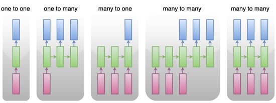
Figure 1. RNN for Variable Inputs/Outputs.
The cases presented in Figure 1 may be summarized in the following three categories.
-
One to Many, applied in fields of image captioning, text generation
-
Many to One, applied in fields of sentiment analysis, text classification
-
Many to Many, applied in fields of machine translation, voice recognition
However, RNN may deal with the above-mentioned cases as it includes a recursive processing unit with single or multiple layers of cells) plus a hidden state extracted from past data.
The use of a recursive processing unit has advantages and disadvantages. The main advantage is that the network may handle inputs and outputs of varied sizes. Unfortunately, the main disadvantages are the difficulty of storing past data and the complication of vanishing/exploding gradients.
3. Vanilla RNN
A Vanilla RNN is a type of neural network that can process sequential data, such as time-series data or natural language text, by maintaining an internal state. In a vanilla RNN, the output of the previous time step is fed back into the network as input for the current time step, along with the current input. This allows the network to capture information from previous inputs and use it to inform the processing of future inputs. The term “vanilla” is used to distinguish this type of RNN from more complex variants, such as LSTMs (Long Short-Term Memory) and GRUs (Gated Recurrent Units), which incorporate additional mechanisms to better handle long-term dependencies in sequential data. Despite their simplicity, vanilla RNNs can be effective for a range of tasks, such as language modeling, speech recognition, and sentiment analysis. However, they can struggle with long-term dependencies and suffer from vanishing or exploding gradients, which can make training difficult. In Figure 2 the main RNN architecture incorporating self-looping or recursive pointer is presented. Let us consider input, output, and hidden state as x, o, and h, respectively, while U, W, and V are the corresponding parameters. In this architecture, an RNN cell (in green) may include one or more layers of normal neurons or other types of RNN cells.
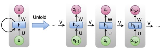
Figure 2. Basic RNN architecture.
The main concept of RNN is the recursive pointing structure which is based on the following rules:
-
Inputs and outputs are of variable size
-
In each stage the hidden state from the previous stage as well as the current input is utilized to compute the current hidden state that feeds the next stage. Consequently, knowledge from past data is transmitted through the hidden states to the next stages. Hence, the hidden state is a means of connecting the past with the present as well as input with output.
-
The set of parameters U, V, and W as well as the activation function are common to all RNN cells.
Unfortunately, the shared among all cells set of parameters (U, V, W) constitutes a serious bottleneck when the RNN raises enough. In this case, a brain consisting of only one set of memory may be overloaded. Therefore, Vanilla RNN cells that have multi-layers may easily enhance the performance.
4. Long Short-Term Memory
LSTM networks are a type of RNN designed to handle long-term dependencies in data. LSTMs were first introduced by Hochreiter and Schmidhuber in 1997 and have since become widely used due to their success in solving a variety of problems. Unlike standard RNNs, LSTMs are specifically created to address the issue of long-term dependency, making it their default behavior.
LSTMs consist of a chain of repeating modules, similar to all RNNs, but the repeating module in LSTMs is structured differently. Instead of a single layer, LSTMs have four interacting layers. The key component of LSTMs is the cell state, a horizontal line that runs through the modules and enables an easy flow of information. The LSTMs regulate the flow of information in the cell state through gates, which consist of a sigmoid neural network layer and a pointwise multiplication operation. The sigmoid layer outputs numbers between 0 and 1 to determine the amount of information to let through.
LSTMs have three gates to control the cell state: the forget gate, the input gate, and the output gate. The forget gate uses a sigmoid layer to decide which information to discard from the cell state. The input gate consists of two parts: a sigmoid layer that decides which values to update, and a tanh layer that creates new candidate values. The new information is combined with the cell state to create an updated state. Finally, the output gate uses a sigmoid layer to decide which parts of the cell state to output, then passes the cell state through tanh and multiplies it by the output of the sigmoid gate to produce the final output.
5. Convolutional Neural Network
CNN [36] is a type of deep learning neural network commonly used in image recognition and computer vision tasks. It is based on the concept of convolution operation, where the network learns to extract features from the input data through filters or kernels. The filters move over the input data and detect specific features such as edges, lines, patterns, and shapes, which are then processed and passed through multiple layers of the network. These multiple layers allow the CNN to learn increasingly complex representations of the input data. The final layer of the CNN outputs predictions for the input data based on the learned features. In addition to image recognition, CNNs can be applied to various other tasks including natural language processing, audio processing, and video analysis.
6. Gated Recurrent Unit
The GRU [38] operates similarly to an RNN, but with different operations and gates for each GRU unit. To address issues faced by standard RNNs, GRUs incorporate two gate mechanisms: the Update gate and the Reset gate. The Update gate determines the amount of previous information to pass on to the next stage, enabling the model to copy all previous information and reduce the risk of vanishing gradients. The Reset gate decides how much past information to ignore, deciding whether previous cell states are important. The Reset gate first stores relevant past information into a new memory then multiplies the input and hidden states with their weights, calculates the element-wise multiplication between the Reset gate and the previous hidden state, and applies a non-linear activation function to generate the next sequence.
This entry is adapted from the peer-reviewed paper 10.3390/technologies11030070
This entry is offline, you can click here to edit this entry!