Your browser does not fully support modern features. Please upgrade for a smoother experience.
Please note this is an old version of this entry, which may differ significantly from the current revision.
Subjects:
Engineering, Manufacturing
|
Engineering, Industrial
|
Computer Science, Artificial Intelligence
The advancement of Industry 4.0 and smart manufacturing has made a large amount of industrial process data attainable with the use of sensors installed on machines. This stands true for Industrial Dryer Hoppers, which are used for most polymer manufacturing processes. Insights derived via AI from the collected data allow for improved processes and operations.
- industry 4.0
- smart manufacturing
- machine learning
- deep learning
1. Introduction
The advancement of smart manufacturing, which combines information technology and operational technology, has enabled the collection and processing of large amounts of industrial process data [1]. This progress has been facilitated by the installation of numerous sensors in industrial equipment and machine tools on the shop floor, leading to an increase in available data. In many cases, these sensors record the activity of manufacturing machine tools over time, thus generating time-series data [2]. The analysis of time-series data has proven valuable in extracting meaningful events in smart manufacturing systems [3]. While time-series data can be found in various domains such as healthcare [4], climate [5], robotics [6], ecohydrology [7], stock markets [8], energy systems [9], etc.
Sensors play a crucial role in the advancement of smart manufacturing systems, collecting data for various key variables over time, and forming Multivariate Time-Series (MTS) data. MTS data consists of multiple univariate time series (UTS), making MTS more complex due to the correlation between different variables. This paper focuses on the analysis of time-series data for classification, which involves identifying key events and their respective classes within a dataset. Classification models aim to categorize events based on specific patterns and assign them to corresponding categories. In MTS classification, the time series is divided into segments, each belonging to a category with distinct patterns.
Several algorithms have been developed to analyze MTS data. Traditional approaches used prior to the evolution of smart manufacturing include simple exponential smoothing [11], dynamic time warping [12,13], and autoregressive integrated moving averages [14]. Machine learning algorithms such as K-nearest neighbor [15], decision trees [16], and Support Vector Machine (SVM) [17] have also been employed. Some authors have combined the K-nearest neighbor with distance measures like DTW [18,19] or Euclidean distance [20,21]. It has been shown that ensembling different discriminant classifiers, such as SVM and nearest neighbor, along with other machine learning classifiers like decision trees and random forests, can yield better results than using nearest neighbor with dynamic time warping [12]. Traditional methods often struggle to identify important features within time-series data and fail to capture correlations between variables, leading to the false identification of categorical events [3]. Additionally, traditional approaches and machine learning algorithms face challenges in handling the massive volume of data. Deep learning, with its ability to handle large amounts of data using deep neural networks, has emerged as a solution for extracting meaningful features from MTS data.
Deep learning techniques, including various neural network algorithms, have gained significant attention in dealing with time-series problems, particularly MTS. Deep neural networks can learn patterns in the data by capturing the correlations between variables, surpassing traditional methods such as NN-DTW. While NN-DTW may perform well for a small number of variables, it becomes more complex as the number of variables increases [22]. In this paper’s case study, which involves twelve distinct temperature measures, deep neural networks are particularly relevant. The two most used neural networks are Convolutional Neural Networks (CNN) and Recurrent Neural Networks (RNN). CNNs are popular for computer vision tasks [23] and have been extensively applied to image recognition [24], natural language processing [25,26,27], image compression, and speech recognition [28]. CNNs have also been successful in handling MTS problems [3,22,29,30,31,32,33,34]. RNN, on the other hand, excels in sequential learning and performs well for univariate time series, but its application to MTS classification is limited [35]. However, it shows promise in dealing with time-series datasets containing missing values [36].
2. Manufacturing Process
In the polymer processing industry, dryers play a crucial role in supplying dry-heated air that is blown upward through the to-be-dried material for several hours, while new undried, cold/moist material is continuously loaded on top of the dryer module, steadily moving downward through the dryer [37,38]. Modern drying hoppers are designed with a cylindrical body and a conical hole at the bottom. They ensure even temperature distribution and material flow by using spreader tubes to inject hot and dry air into the chamber. The process involves recirculating the hot air to continuously dry the material until the desired humidity level is achieved. Successful drying requires considering three main factors: drying time, drying temperature, and the dryness of circulating air. Drying time depends on the air temperature, initial dryness of the material, and target humidity. Higher air dryness and temperature accelerate the drying process, but excessively high temperatures may affect the material’s quality [39].
Monitoring the drying process is essential to avoid malfunctions. In a typical use case, a six-zoned temperature probe continuously measures the temperature at different heights within the vertically aligned drying chamber. This helps detect various disruptions in the drying process, such as over- or under-dried material and heater malfunctions [39]. The drying hopper consists of a drying hopper monitor and a regen wheel, both of which have a significant impact on polymer processing. The drying hopper monitor has eight temperature sensors, while the regen has three temperature sensors, including dew point temperature measurements for air delivery. Temperature sensors are used to measure these twelve temperatures over a period of one year for this specific case study. Figure 1 depicts a schematic of a drying hopper and sensor setup similar to the one used in this study.
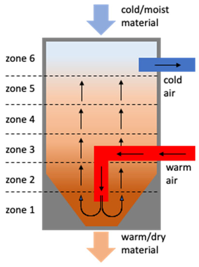
Figure 1. A view of a drying hopper with different temperature zones.
The collected data are preprocessed by handling missing values, outliers, and extraneous cases. The dataset contains temperature readings for twelve temperature measures sampled at one-minute intervals over the course of a year. With a large amount of data available for the main temperature zones in the dryer/hopper system and additional zones in the regen and dryer regions, meaningful features can be extracted via real-time analysis. By analyzing these data in real time, the production planner can gain insights into the drying hopper’s performance and determine the necessary maintenance actions. Figure 2 shows the temperature profiles obtained from the sensors.
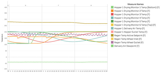
Figure 2. The temperature profile of the data gathered from the case study drying hopper.
3. Time-Series Classification in Manufacturing—Algorithms
MTS has gained popularity across various domains for different purposes, including clinical diagnosis, weather prediction, stock price analysis, human motion detection, and fault detection in manufacturing processes. The manufacturing industry, in particular, has seen a significant increase in the use of MTS data due to the deployment of sensor systems in shop-floor machinery and machine tools. As a result, researchers in the manufacturing domain have focused on MTS analysis, such as classification, to address the challenges posed by these data. Temporal data mining, including MTS analysis, presents complexities arising from factors like spatial structure, time dependency, and correlations among variables. Consequently, researchers have been developing a variety of algorithms to handle these challenges.
3.1. Traditional Algorithms
The K-nearest neighbor algorithm with Dynamic Time Warping (DTW) is commonly used as a benchmark for classifying MTS data. In ref. [40], the authors used the Large Margin Nearest Neighbor (LMNN) and DTW. Mahalanobis distance-based DTW is used to calculate the relations among variables using the Mahalanobis matrix and LMNN is used to learn the matrix by minimizing a renewed, non-differentiable cost function using the coordinate descent method. This method is compared with other similarity measure techniques of MTS and the authors claimed the superiority of their proposed method over other techniques. This technique is also used by the authors in [41]. DTW multivariate prototyping is used in evaluating scoring and assessment methods for virtual reality training simulators. It classifies the VR data as novice, intermediate, or expert where 1-NN DTW performed reasonably well; the only better algorithm for this case was RESNET, which is an advanced version of CNN [42]. Overall, using DTW as a dissimilarity measure among features of time series and adapting the nearest neighbor classifier in temporal data mining was very popular before the evolution of deep learning [43].
According to [38], there are two approaches that can be taken for MTS data using DTW. One approach involves summing up the DTW distances of UTS for each dimension of the MTS. The other approach calculates the distance between two time-series data by summing up the distances between each corresponding pair of time-series data. The authors argue that the traditional belief that these two methods are equivalent for MTS classification is not true, and their effectiveness varies depending on the specific case. They conducted experiments on a wide range of MTS datasets to support their claim and justify the use of different DTW approaches based on the problem at hand.
A parametric derivative DTW is another variant of the DTW used in temporal data mining. This technique combines two distances, which are the DTW distance between MTS and the DTW distance between derivatives of MTS. This new distance is used afterward for classification with nearest neighbor rules [44]. Using a template selection approach based on DTW so that the complex feature selection approach and domain knowledge can be avoided is another approach used for classifying MTS in [45]. Another variant of DTW is using DTW distance measured via integral transformation. Integral DTW is calculated as the value of DTW on the integrated time series. This technique combines the DTW and integral DTW with the 1-nearest neighbor classifier which shows no overfitting issue [46].
The symbolic representation of MTS is a traditional technique used for classification. It involves learning symbols using supervised learning algorithms, considering all elements of the time series simultaneously. Tree-based ensembles are utilized to detect interactions between UTS columns, enabling efficient handling of nominal and missing values [47]. Another symbolic representation technique is MrSEQL, which transforms the time-series data using symbolic aggregate approximation (SAX) [48] in the time domain and symbolic Fourier approximation (SFA) [49] in the frequency domain. Discriminative subsequences are extracted from the symbolic data and used as features for training a classification model [50,51]. WEASEL + MUSE is another approach that uses SFA transformation to create sequences of words. Feature selection is performed using a chi-squared model, and logistic regression is employed to learn the selected features. These symbolic representation methods provide alternatives to traditional DTW-based approaches in MTS classification tasks [52].
One of the most extensive research on traditional methods for both MTS and UTS can be found in [12], which highlights almost all of the above-mentioned traditional approaches in different categories like whole series similarity, phase-dependent intervals, phase-independent shapelets, dictionary-based classifiers, and combinations of transformations. This paper is a great resource for any time-series classification enthusiast to gain an overview of all the traditional methods. Another review paper that shows a brief overview of different classification approaches for MTS can be found in [51].
Machine learning algorithms, including both nonlinear techniques and ensemble learning techniques, have also been applied for time-series classification over the years. Traditional classifiers like Naïve Bayes, Decision Tree, and SVM are the most popular. Before using these algorithms, MTS data need to be converted into feature vector format. This is why the authors in [17] segmented the time series to obtain a qualitative description of each series and determined the frequent patterns. Afterward, the patterns that are highly discriminative between the classes are selected, and the data are transformed into vector format where the features are discriminative patterns.
3.2. Deep Learning Algorithms
ANN and deep learning, specifically Convolutional Neural Networks (CNN) and Recurrent Neural Networks (RNN) such as Long Short-Term Memory (LSTM), have gained significant popularity in the field of temporal data mining, particularly for time-series classification. CNN has been widely used with a 1D filter in the convolutional layer, allowing it to automatically discover and extract meaningful internal structures in input time series via convolution and pooling operations. This eliminates the need for manual feature engineering, which is typically required in traditional feature extraction methods [53]. The combination of CNN and LSTM, leveraging the strengths of both algorithms, has also shown excellent performance in time-series classification tasks. Researchers have proposed various versions and adaptations of these algorithms, each showing promising results in different case studies. The authors of [22,54] provided the summary and basics of the recent algorithmic advance in the use of deep learning for MTS classification.
The authors in [29] used a tensor scheme with multivariate CNN for the time-series classification where the model considers multivariate aspect and lag feature characteristics simultaneously. Four stages were used in CNN architecture, which are the input tensor transformations stage, univariate convolution stage, multivariate convolution stage, and fully connected stage. In this method, they used an image-like tensor scheme to encode the MTS data. This approach is taken because of the highly successful nature of CNN in computing the vision for image classification.
Deconvolution has been utilized in time-series data mining, in addition to the convolution operation. In a study [55], the authors employed a deconvolutional network combined with SAX discretization to learn the representation of MTS. This approach captured correlations using deconvolution and applied pooling operations for dimension reduction across each position of each variable. SAX discretization was used to extract a bag of features, resulting in improved classification accuracy. Another variation of CNN called dilated CNN treated MTS as an image and employed stacks of dilated and stridden convolutions to extract features across variables [31]. Among other CNN approaches, multi-channel deep CNN is widely utilized, where the model learns features from individual time series and combines them after the convolution and pooling stages. The combined features are then fed into a multilayer perceptron (MLP) for final classification [34].
In [56], the authors performed a principal component analysis for feature extraction and reduced the number of MTS variables to two so that they could identify the most useful two components in the machine. The time series are encoded into images using Gramian Angular field (GAF) and the images are used as input for the CNN. Another similar research can be found in [57] where three techniques of converting MTS data into images have been used and tested, which are GAF, Gramian Angular Difference Field (GADF), and Markov Transition Field (MTF). It has been found that different approaches to converting MTS into images do not affect the classification performance, and a simple CNN can outperform other approaches. In semiconductor manufacturing, it has been tested that MTS- CNN can successfully detect fault wafers with high accuracy, recall, and precision [3].
Combining CNN, LSTM, and DNN has been another highly used approach over the years. In [58], the authors proposed a combined architecture abbreviated as CLDNN and applied it to large vocabulary tasks which outperformed three individual algorithms. A similar approach named MDDNN has been used to predict the class of a subsequence in terms of earliness and accuracy. The attention mechanism is incorporated with the deep learning framework in order to identify critical segments related to model performance [59]. The proposed framework used both the time domain and frequency domain via fast Fourier transformation and merged them for prediction. Another similar research that focused on early classification can be found in [30].
Apart from LSTM, other recurrent network variants like bidirectional RNN (BiRNN), bidirectional Long Short-Term Memory (BiLSTM), Gated Recurrent Unit (GRU), Bidirectional Gated Recurrent Unit (BiGRU) have been adapted to use in MTS classification. In [60], the authors used MLSTM-FCN, which is the combination of LSTM, squeeze and excitation (SE) block, and CNN, in which the SE block is integrated within FCN to leverage its high performance for MTS classification. A similar approach of using an excitation block has also been used in [32].
Multi-scale entropy and inception structure ideas have been used with the LSTM-FCNN model for MTS classification. The subsequences of each variable have been convolved using a 1D convolutional kernel with different filter sizes to extract high-level multi-scale spatial features. Afterward, LSTM has been applied to further process and capture temporal information. Both these spatial and temporal features are used as input to the fully connected layer [33]. In addition to CNN, the Evidence Feed Forward Hidden Markov Model (EFF-HMM) has been combined with LSTM to classify MTS. According to [61], learning EFF-HMM is based on the mistakes of the LSTM that outperformed other state of the art in human activity recognition.
This entry is adapted from the peer-reviewed paper 10.3390/jmmp7050164
This entry is offline, you can click here to edit this entry!