Optimal Design of Neural Networks Based on FPGA

Optimal Design of Neural Networks Based on FPGA: History

View Latest Version

Please note this is an old version of this entry, which may differ significantly from the current revision.

Subjects: Computer Science, Hardware & Architecture

Contributor:

Chenghao Wang

Zhongqiang Luo

基于神经网络的深度学习已广泛应用于图像识别、语音识别、自然语言处理、自动驾驶等领域，并取得了突破性进展。FPGA以其灵活的架构和逻辑单元、高能效比、强兼容性、低时延等优势在加速深度学习领域脱颖而出。

deep learning
deep neural network
FPGA

1. Introduction

With the rise of the short video industry and the advent of the era of big data and the Internet of Things (IoTs), the data created by people in recent years has shown a blowout growth, providing a solid data foundation for the development of artificial intelligence (AI). As the core technology and research direction for realizing artificial intelligence, deep learning based on neural networks has achieved good results in many fields, such as speech recognition [1,2,3], image processing [4,5,6], and natural language processing [7,8,9]. Common platforms to accelerate deep learning include central processing unit (CPU), graphics processing unit (GPU), field-programmable gate array (FPGA), and application-specific integrated circuit (ASIC).

Among them, the CPU adopts Von Neumann architecture and the program execution in the field of deep learning of artificial intelligence is less, while the computational demand for data is relatively large. Therefore, the implementation of AI algorithms by CPU has a natural structural limitation—that is, the CPU spends a large amount of time reading and analyzing data or instructions. In general, it is not possible to achieve unlimited improvement of instruction execution speed by increasing CPU frequency and memory bandwidth without limit.

The ASIC special purpose chip has the advantages of high throughput, low latency, and low power consumption. Compared with FPGA implementation of the same process, ASIC can achieve 5~10 times the computation acceleration, and the cost of ASIC will be greatly reduced after mass production. But, deep learning computing tasks are flexible, each algorithm’s needs can be implemented effectively through slightly different dedicated hardware architecture, and there is a high cost of research and development of ASIC and flow, with the cycle being long, yet the most important thing to note is that is logic cannot cause dynamic adjustment, which means that the custom accelerator chips (such as ASIC) must make a large amount of compromise in order to act as a sort of universal accelerator.

At a high level, this means that system designers face two choices. One is to select a heterogeneous system and load a large number of ASIC accelerator chips into the system to deal with various types of problems. Or, one can choose a single chip to handle as many types of algorithms as possible. The FPGA scheme falls into the latter category because FPGA provides unlimited reconfigurable logic, whereas FPGA can update the logic function in only a few hundred milliseconds.

At present, artificial intelligence computing requirements represented by deep learning mainly use GPU, FPGA, and other existing general chips that are suitable for parallel computing in order to achieve acceleration. Due to the characteristics of high parallelism, high frequency, and high bandwidth, GPU can parallelize the operation and greatly shorten the operation time of the model. Due to its powerful computing ability, it is mainly used to deal with large-scale computing tasks at present. GPU-accelerated deep learning algorithms have been widely used and have achieved remarkable results.

Compared with FPGA, the peak performance of GPU (10 TFLOPS, floating point operation per second) is much higher than that of FPGA (<1 TFLOPS), and thus GPU is a good choice for deep learning algorithms in terms of accelerating performance. However, this is only the case when the power consumption is not considered. Because the power consumption of GPU is very high, sometimes tens of hundreds of times that of CPU and FPGA, the high energy consumption limits it to being used in high-performance computing clusters. If it is used on edge devices, the performance of GPU will be greatly sacrificed.

However, the DDR (double data rate) bandwidth, frequency, and number of computing units (low-end chips) of FPGA are not as high as GPU. For on-chip memory, FPGA has larger computing capacity; moreover, on-chip memory is crucial for reducing latency in applications such as deep learning. Accessing external memory such as DDR consumes more energy than the chip itself for computing. Therefore, the larger capacity of on-chip cache reduces the memory bottleneck caused by external memory reading and also reduces the power consumption and cost required by high-memory bandwidth. The large capacity of on-chip memory and flexible configuration capability of FPGA reduces the read and write of external DDR, while GPU requires the support of an external processor during operation. The addition of external hardware resources greatly reduces the data processing speed. Moreover, FPGA’s powerful raw data computing power and reconfigurability allow it to process arbitrary precision data, but GPU’s data processing is limited by the development platform. Therefore, in this context, FPGA seems to be a very ideal choice. In addition, compared with GPU, FPGA not only has the characteristics of data parallel, but also has the characteristics of pipeline parallel, and thus for pipelined computing tasks, FPGA has a natural advantage in delay. On the basis of these advantages, FPGA stands out in the field of accelerated deep learning.

In the previous work, the application, acceleration method and accelerator design of neural networks such as CNN (convolutional neural network), RNN (recurrent neural network), and GAN (generative adversarial network) based on FPGA were described in detail, and the research hotspots of industrial application combined with FPGA and deep neural networks were fully investigated. They have made relevant contributions to the application and development of FPGA in neural networks [10,11,12,13,14]. It is worth noting that the analysis of the acceleration effect of different acceleration techniques on different neural networks is less involved in their work.

2. The Development of Neural Networks

As shown in Table 1, the development process of neural networks can be roughly divided into five stages: the proposal of the model, the stagnation period, the rise of the back propagation algorithm, the confusion period, and the rise of deep learning.

Table 1. Development history of neural networks.

Stage	Year	Character	Content
Generation of models	1943	Warren McCulloch and Walter Pitts	McCulloch–Pitts model [15]
	1948	Alan Mathison Turing	B-type Turing machine [16]
	1949	Donald Hebb	Hebb algorithm [17]
	1951	McCulloch and Marvin Minsky	The first neural network machine SNARC
	1958	Frank Rosenblatt	Perceptron model [18]
Lag phase	1969	Marvin Minsky	Perception [19]
	1974	Paul J. Werbos	Backpropogation (BP) algorithm [20]
	1980	Kunihiko Fukushima	Neocognitron model [21]
The rise of backpropagation algorithms	1982	John J. Hopfield	Hopfield model [22]
	1985	Hinton and Sejnowski	Boltzmann machine [23]
	1986	David Rumelhart and James McClelland	Redescription of the BP algorithm [24]
	1989	LeCun	Introducing the BP algorithm to the convolutional neural network [25]
Confusion period	1990–2005	The rise of machine learning models has brought about great challenges to the development of neural networks
The rise of deep learning	2006	Geoffrey Hinton	Deep Belief Networks [26]
	2012	Alex Krizhevsky	AlexNet [27]
	2014	Christian Szegedy	GoogLeNet [28]
		Visual Geometry Group and Google DeepMind	VGGNet [29]
		Ian J. Goodfellow	GAN [30]
		Yi Sun and Xiaogang Wang	DeepID [31]
		Ross Girshick and Jeff Donahue	Region-CNN (RCNN) [32]
	2015	Joseph Redmon	You Only Look Once (YOLOv1) [33]
	2016	AlphaGo, an artificial intelligence machine developed by Google’s DeepMind, beat Go world champion Lee Sedol 4-1
	2016	Joseph Redmon	YOLOv2 [34]
	2018	Joseph Redmon	YOLOv3 [35]
	2020	Alexey Bochkovskiy	YOLOv4 [36]
	2020–2022	YOLOv5, YOLOv6 [37], YOLOv7 [38], etc.

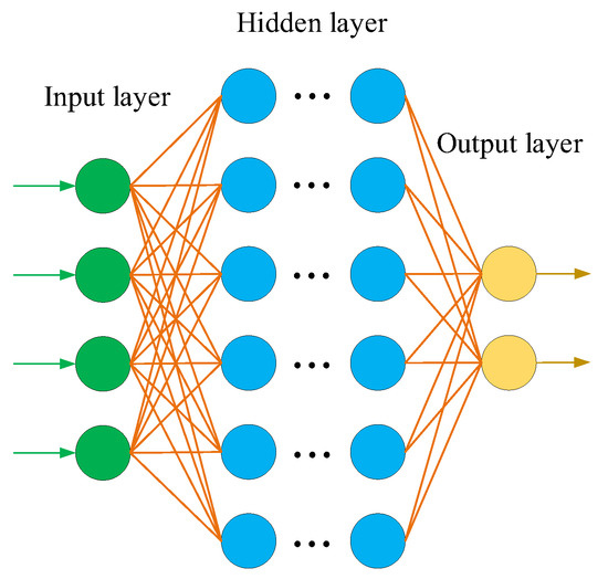
2.1. Deep Neural Network (DNN)

Since a single-layer perceptron cannot solve linear inseparability problems, it cannot be used in industry. Scholars have expanded and improved the perceptron model by increasing the number of hidden layers and corresponding nodes to enhance the expression ability of the model, and thus the deep neural network (DNN) was created. The DNN is sometimes called a multi-layer perceptron (MLP). The emergence of the DNN overcomes the low performance of a single-layer perceptron. According to the position of different layers in the DNN, the neural network layers inside the DNN can be divided into three types: the input layer, hidden layer, and output layer, as shown in Figure 2.

Figure 2. Typical model of a DNN.

2.2. Convolutional Neural Network (CNN)

The CNN model was developed from the early artificial neural network. On the basis of the research of Hub et al. on the cells in the visual cortex of cats, the CNN model is a specially designed artificial neural network with multiple hidden layers through the biomimetic brain skin layer. Convolution operation is used to solve the disadvantages of large computation and loss of structure information of artificial neural networks.

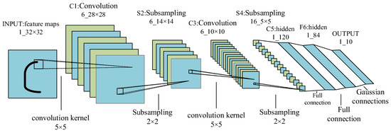
The birth of LeNet-5 established the basic embryonic form of CNN, which is composed of a convolution layer, a pooling layer, an activation function, and a fully connected layer connected in a certain number of sequential connections, as shown in Figure 3. The CNN is mainly applied to image classification [39,40,41], object detection [42,43], and semantic segmentation [44,45,46], as well as in other fields. The most common algorithms are YOLO and R-CNN, among which YOLO has a faster recognition speed due to the characteristics of the algorithm. It has been upgraded to V7. R-CNN’s target location search and identification algorithm are slightly different from those of YOLO. Although the speed is slower than that of YOLO, the accuracy rate is higher than that of YOLO.

Figure 3. The Lenet-5 model.

2.3. Recurrent Neural Network (RNN)

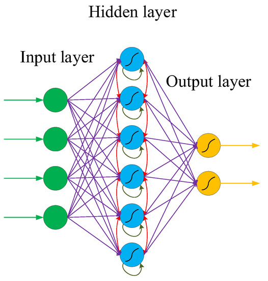
Different from CNN, RNN introduces the dimension of “time”, which is suitable for processing time-series-type data. Because the network itself has a memory ability, it can learn data types with correlation before and after. Recurrent neural networks have a strong model fitting ability for serialized data and are widely used in the field of natural language processing (NLP), including image classification, image acquisition, machine translation, video processing, sentiment analysis, and text similarity calculation. The specific structure is as follows: the recurrent neural network will store and remember the previous information in the hidden layer and then input it into the current calculation of the hidden layer unit.

Figure 4 shows the typical structure of an RNN, which is similar to but different from the traditional deep neural network (DNN). The similarity lies in that the network models of DNN and RNN are fully connected from the input layer to the hidden layer and then to the output layer, and the network propagation is also sequential. The difference is that the internal nodes of the hidden layer of the RNN are no longer independent of each other but have messages passing to each other. The input of the hidden layer can be composed of the output of the input layer and the output of the hidden layer at a previous time, which indicates that the nodes in the hidden layer are self-connected. It can also be composed of the output of the input layer, the output of the hidden layer at the previous moment, and the state of the previous hidden layer, which indicates that the nodes in the hidden layer are not only self-connected but also interconnected.

Figure 4. Typical structure of an RNN.

2.4. Generative Adversarial Network (GAN)

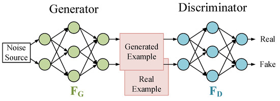
The GAN (generative adversarial network) is a machine learning model designed by Goodfellow et al. [30] in 2014. Inspired by the zero-sum game in game theory, this model views the generation problem as a competition between generators and discriminators. The generative adversarial network consists of a generator and a discriminator. The generator generates data by learning, and the discriminator determines whether the input data are real data or generated data. After several iterations, the ability of the generator and discriminator is constantly improved, and finally the generated data are infinitely close to the real data so that the discriminator cannot judge whether they are true or false. The GAN is shown in Figure 5.

Figure 5. Typical structure of a GAN.

3. Application of Neural Networks Based on FPGA

3.1. Application of CNNs Based on FPGA

In terms of intelligent medical treatment, in November 2019, Serkan Sağlam et al. [47] deployed a CNN on FPGA to classify malaria disease cells and achieved 94.76% accuracy. In 2020, Qiang Zhang et al. [48] adopted a CPU + FPGA heterogeneous system to realize CNN classification of heart sound sample data, with an accuracy of 86%. The fastest time to classify 200 heart sound samples was 0.77 s, which was used in the machine of primary hospital to assist in the initial diagnosis of congenital heart disease.

In terms of national defense, in 2020, Cihang Wang et al. [52] found that a large number of high-precision and high-resolution remote sensing images were used in civil economic construction and military national defense, and thus they proposed a scheme of real-time processing of remote sensing images that was based on a convolutional neural network on the FPGA platform. This scheme optimized CNN on FPGA from two aspects: spatial parallel and temporal parallel. By adding pipeline design and using the ideas of module reuse and data reuse, the pressure of the data cache was reduced, and the resource utilization of FPGA was increased. Compared with other schemes, the proposed scheme greatly improved the recognition speed of remote sensing images, reduced the power consumption, and achieved 97.8% recognition accuracy. Although the scheme uses many speedup techniques, it does not optimize the convolution operation, which has the most significant performance improvement.

3.2. Application of RNNs Based on FPGA

At present, in addition to the application of deep neural networks into the fields of image and video, an FPGA-based speech recognition system has also become a research hotspot. Among them, the commonly used speech recognition model is the RNN and its variant LSTM. Due to its huge market demand, speech recognition develops rapidly. In intelligent speech recognition products, in order to ensure certain flexibility and mobility, the speech recognition model is usually deployed on FPGA to meet the needs of intelligence and production landing.

In 2016, the work of J. C. Ferreira and J. Fonseca et al. [54] was considered as one of the earliest works to implement the LSTM network on the FPGA hardware platform, which focused people’s attention from the software implementation of LSTM to FPGA hardware. In 2017, Y. Guan et al. [55] implemented the LSTM network using special hardware IP containing devices such as data scheduler, FPGA, AXI4Lite (one of the Advanced eXtensible Interfaces) bus, and optimized computational performance and communication requirements in order to accelerate inference.

In 2018, Zhe Li et al. [59] summarized two previous works on the FPGA implementation of the LSTM RNN inference stage on the basis of model compression. One work found that the network structure became irregular after weight pruning. Another involved adding a cyclic matrix to the RNN to represent the weight matrix in order to achieve model compression and acceleration while reducing the influence of irregular networks. On this basis, an efficient RNN framework for automatic speech recognition based on FPGA was proposed, called E-RNN. Compared with the previous work, E-RNN achieved a maximum energy efficiency improvement of 37.4 times, which was more than two times that of the latter work under the same accuracy.

In December of the same year, Chang Gao et al. [62] proposed a lightweight gated recursive unit (GRU)-based RNN accelerator, called EDGERDNN, which was optimized for low-latency edge RNN inference with batch size 1. EDGERDRNN used a delta network algorithm inspired by pulsed neural networks in order to exploit the temporal sparsity in RNN. Sparse updates reduced distributed RAM (DRAM) weight and memory access by a factor of 10, and reduced latency, resulting in an average effective throughput of 20.2 GOP/s for batch size 1.

3.3. Application of GANs Based on FPGA

In 2018, Amir Yazdanbakhsh et al. [66] found that generators and discriminators in GANs use convolution operators differently. The discriminator uses the normal convolution operator, while the generator uses the transposed convolution operator. They found that due to the algorithmic nature of transposed convolution and the inherent irregularity in its computation, the use of conventional convolution accelerators for GAN leads to inefficiency and underutilization of resources. To solve these problems, FlexiGAN was designed, an end-to-end solution that generates optimized synthesizable FPGA accelerators according to the advanced GAN specification. The architecture takes advantage of MIMD (multiple instructions stream multiple data stream) and SIMD (single instruction multiple data) execution models in order to avoid inefficient operations while significantly reducing on-chip memory usage. The experimental results showed that FlexiGAN produced an accelerator with an average performance of 2.2 times that of the optimized conventional accelerator. The accelerator delivered an average of 2.6 times better performance per watt compared to the Titan X GPU.

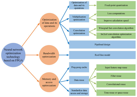
4. Neural Network Optimization Technology Based on FPGA

With the rapid development of artificial intelligence, the number of layers and nodes of neural network models is increasing, and the complexity of the models is also increasing. Deep learning and neural networks have put forward more stringent requirements on the computing ability of hardware. On the basis of the advantages of FPGA mentioned in the introduction, increasingly more scholars are choosing to use FPGA to complete the deployment of neural networks. As shown in Figure 6, according to different design concepts and requirements, FPGA-based neural network optimization technology can be roughly divided into optimization for data and operation, optimization for bandwidth, and optimization for memory and access, among others, which are introduced in detail below.

Figure 6. Neural network optimization technology based on FPGA.(fixed-point quantization [71,72,73,74,75,76,77,78], less computations [79,80,81], improve calculation speed [82,83,84,85], Winograd fast convolution algorithm [86,87,88,89,90,91], Im2col convolution optimization algorithm [92,93,94,95,96,97], pipelined design [98,99,100,101,102], Roof-line model [103,104,105], ping-pong cache [106,107,108,109], input feature map reuse [110,111], filter reuse [111,112], convolutional reuse [110,111,112], time reuse or space reuse [111], standardize data access and storage [113,114,115]).

4.1. Optimization of Data and Its Operations

In the aspect of optimization of data and its operation, scholars have made many attempts and achieved certain results. Aiming at the data itself, a method to reduce the data accuracy and computational complexity is usually used. For example, fixed-point quantization is used to reduce the computational complexity with an acceptable loss of data accuracy, so as to improve the computational speed. In terms of operation, the optimization is realized by reducing the computation times of multiplication and increasing the computation speed. The commonly used optimization methods include addition calculation instead of multiplication calculation, the Winograd fast convolution algorithm, and the Im2col convolution acceleration algorithm, among others.

4.1.1. Fixed-Point Quantitative

Since the bit width of the number involved in the operation is finite and constant in FPGA calculations, the floating-point decimal number involved in the operation needs to be fixed to limit the bit width of a floating-point decimal to the range of bit width allowed by FPGA. Floating-point decimals mean that the decimal point position is not fixed, and fixed-point decimals mean that the decimal point position is fixed. Fixed-point quantization is the use of finite digits to represent infinite precision numbers, that is, the quantization function maps the full precision numbers (the activation parameters, weight parameters, and even gradient values) to a finite integer space. Fixed-point quantization can greatly reduce the memory space of each parameter and the computational complexity within the acceptable accuracy loss range, so as to achieve neural network acceleration.

In 2011, Vincent Vanhoucke first proposed the linear fixed-point 8-bit quantization technology, which was initially used in X86 CPU, greatly reducing the computational cost, with it then being slowly applied to FPGA [71]. In March 2020, Shiguang Zhang et al. [72] proposed a reconfigurable CNN accelerator with an AXI bus based on advanced RISC machine (ARM) + FPGA architecture.

In June of the same year, Zongling Li et al. [73] designed a CNN weight parameter quantization method suitable for FPGA, different from the direct quantization operation in the literature [72]. They transformed the weight parameter into logarithm base 2, which greatly reduced the quantization bit width, improved the quantization efficiency, and reduced the delay. Using a shift operation instead of a convolution multiplication operation saves a large number of computational resources.

4.1.2. Multiplication Optimization

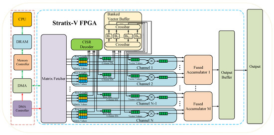
Matrix operations mainly appear in the training and forward computation of neural networks and they occupy a dominant position; thus, it is of great significance to accelerate matrix operation. The optimization of matrix multiplication can be achieved by reducing the number of multiplication computations and increasing the computation speed. Matrix operations often have remarkable parallelism. Scholars usually use the characteristics of FPGA parallel computing to optimize matrix operations.

As shown in Figure 7, the architecture uses specialized compressed interleave sparse row (CISR) coding to efficiently process multiple rows of the matrix in parallel, combined with a caching design that eliminates the replication of the buffer carrier and enables larger vectors to be stored on the chip. The design maximizes the bandwidth utilization by organizing the data from memory into parallel channels, which can keep the hardware complexity low while greatly improving the parallelism and speed of data processing.

Figure 7. Neural network optimization technology based on FPGA.

4.1.3. Convolution Optimization

For the optimization of convolution algorithms, scholars have provided the following two ideas. One is the Winograd fast convolution algorithm, which speeds up convolution by increasing addition and reducing multiplication. Another is the Im2col convolution optimization algorithm that sacrifices storage space in order to improve the speed of the convolution operation.

4.1.4. Pipelined Design

Pipelined design is a method of systematically dividing combinational logic, inserting registers between the parts (hierarchies), and temporarily storing intermediate data. The purpose is to decompose a large operation into a number of small operations. Each small operation takes less time, shortens the length of the path that a given signal must pass in a clock cycle, and improves the frequency of operations; moreover, small operations can be executed in parallel and can improve the data throughput.

The design method of Pipeline can greatly improve the working speed of the system. This is a typical design approach that converts “area” into “velocity”. The “area” here mainly refers to the number of FPGA logic resources occupied by the design, which is measured by the consumed flip-flop (FF) and look-up table (LUT). “Speed” refers to the highest frequency that can be achieved while running stably on the chip. The two indexes of area and speed always run through the design of FPGA, which is the final standard of design quality evaluation. This method can be widely used in all kinds of designs, especially the design of large systems with higher speed requirements. Although pipelining can increase the use of resources, it can reduce the propagation delay between registers and ensure that the system maintains a high system clock speed. In the convolutional layer of deep neural networks, when two adjacent convolutional iterations are performed and there is no data dependency, pipelining allows for the next convolutional operation to start before the current operation is completely finished, improving the computational power, with pipelining having become a necessary operation for most computational engine designs. In practical application, considering the use of resources and the requirements of speed, the series of pipelines can be selected according to the actual situation in order to meet the design needs.

4.2. Bandwidth Optimization

In the deployment of neural networks, all kinds of neural networks must rely on specific computing platforms (such as CPU/GPU/ASIC/FPGA) in order to complete the corresponding algorithms and functions. At this point, the “level of compatibility” between the model and the computing platform will determine the actual performance of the model. Samuel Williams et al. [103] proposed an easy-to-understand visual performance model, the roof-line model, and proposed a quantitative analysis method using operational intensity. The formula showcasing that the model can reach the upper limit of the theoretical calculation performance on the computing platform is provided. It offers insights for programmers and architects in order to improve the parallelism of floating-point computing on software and hardware platforms and is widely used by scholars to evaluate their designs on various hardware platforms to achieve better design results.

The roof-line model is used to measure the maximum floating point computing speed that the model can achieve within the limits of a computing platform. Computing power and bandwidth are usually used to measure performance on computing platforms. Computing power is also known as the platform performance ceiling, which refers to the number of floating pointed operations per second that can be completed by a computing platform at its best, in terms of FLOP/s or GLOP/s. Bandwidth is the maximum bandwidth of a computing platform. It refers to the amount of memory exchanged per second (byte/s or GB/s) that can be completed by a computing platform at its best. Correspondingly, the computing intensity limit Imax is the computing power divided by the bandwidth. It describes the maximum number of calculations per unit of memory exchanged on the computing platform in terms of FLOP/byte.

In recent years, many application achievements based on the roof-line model are also involved in the optimization design of neural networks that are based on FPGA. In 2020, Marco Siracusa et al. [104] focused on the optimization of high-level synthesis (HLS). They found that although advanced synthesis (HLS) provides a convenient way to write FPGA code in a general high-level language, it requires a large amount of effort and expertise to optimize the final FPGA design of the underlying hardware, and therefore they proposed a semi-automatic performance optimization method that was based on the FPGA-based hierarchical roof line model. By combining the FPGA roof-line model with the Design Space Exploration (DSE) engine, this method is able to guide the optimization of memory limit and can automatically optimize the design of a calculation limit, and thus the workload is greatly reduced, and a certain acceleration performance can be obtained.

4.3. Memory and Access Optimization

Data storage and access is an essential part of neural networks. A large amount of data will occupy limited memory space. At the same time, a large amount of memory access will greatly increase the execution time of network models and reduce the computational efficiency. In the aspect of memory and access optimization, ping-pong cache, data reuse, standard data access, and so on are usually used for optimization.

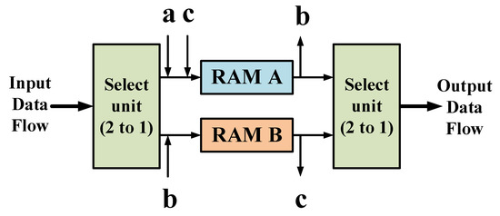
4.3.1. Ping-Pong Cache

The ping-pong cache is a commonly used data flow control technique, which is used to allocate the input data flow to two random access memory (RAM) buffers in equal time through the input data selection unit and realize the flow transmission of data by switching between the two RAM reads and writes.

As shown in Figure 10, a~c describes the complete operation process of completing the cache of data in RAM A and B and the output of data. Each letter represents the input and output of data at the same time, the inward arrow represents the cache of data, and the outward arrow represents the output data. The specific caching process is as follows: The input data stream is allocated to two data buffers in equal time through the input data selection unit, and the data buffer module is generally RAM. In the first buffer cycle, the input data stream is cached to the data buffer module RAM A. In the second buffer cycle, the input data stream is cached to the data buffer module RAM B by switching the input data selection unit, and the first cycle data cached by RAM A is transmitted to the output data selection unit. In the third buffer cycle, the input data stream is cached to RAM A, and the data cached by RAM B in the second cycle is passed to the output data selection unit through another switch of the input data selection unit.

Figure 10. Ping-pong cache description.

4.3.2. Data Reuse

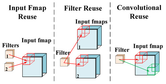
Data reuse is simply the reuse of data. As can be seen from the roof-line model, when the data reuse rate was low, bandwidth became the bottleneck affecting performance, and the computing resources of FPGA were not fully utilized. Therefore, through data reuse, the actual application bandwidth of memory is greater than the theoretical bandwidth, which increases the upper limit of the bandwidth and also reduces the storage pressure of memory and the amount of data cache and data exchange, so as to reduce the unnecessary time spent.

As shown in Figure 11, in the data operation of neural networks, data reuse is usually divided into input feature map reuse, filter reuse, and convolutional reuse. An input feature map reuse is the reuse of the same input and replacing it with the next input after all the convolution kernels are computed. A filter reuse means that if there is a batch of inputs, the same convolution kernel for the batch is reused and the data are replaced after all the inputs in the batch are calculated. Convolutional reuse uses the natural calculation mode in the convolutional layer and uses the same convolution kernel to calculate the output of different input map positions. In general, these three data reuse modes reuse data at different stages in order to achieve the purpose of increasing performance. Of course, data reuse can also be divided by time reuse and space reuse. For example, if the data in a small buffer is repeatedly used in multiple calculations, it is called time reuse. If the same data are broadcast to multiple PEs for simultaneous calculation, it is called space reuse.

Figure 11. Common data reuse modes.

4.3.3. Standardized Data Access and Storage

A large amount of data operation and frequent data access are the problems that neural networks must encounter when they are deployed on portable systems such as FPGA. In the optimization design of neural networks that are based on FPGA, FPGA is usually used as a coprocessor, that is, the CPU writes the instructions to the memory, and then the FPGA reads and executes the instructions from the memory unit, and following this, writes the calculation results to the memory. Therefore, by standardizing data access, the read and write efficiency of data can be improved, and the actual bandwidth upper limit can be increased.

5. Design of the DNN Accelerator and Acceleration Framework Based on FPGA

In the optimization design of neural networks that are based on FPGA, some FPGA synthesis tools are generally used. The existing synthesis tools (HLS, OpenCL, etc.) that are highly suitable for FPGA greatly reduce the design and deployment time of neural networks, and the hardware-level design (such as RTL, register transfer level) can improve the efficiency and achieve a better acceleration effect. However, with the continuous development of neural networks, its deployment on FPGA has gradually become the focus of researchers. This further accelerates the emergence of more accelerators and acceleration frameworks for neural network deployment on FPGA. This is because with the acceleration of the specific neural network model, the idea is the most direct, and the design purpose is also the clearest. These accelerators are often hardware designs for the comprehensive application of the various acceleration techniques described above. When used in specific situations, such accelerators usually only need to fine-tune the program or parameters to be used, which is very convenient [13].

5.1. FPGA Accelerator Design for Different Neural Networks

With the continuous development of deep learning, neural networks have achieved great success in various fields, such as image, speech, and video, and neural networks are developing towards deeper and more complex network design. The way in which to deploy more complex neural networks on FPGA and meet certain speed requirements has become the focus of researchers. In the existing research, a large number of neural network accelerator designs that are based on FPGA have emerged. The main one is the CNN accelerator that is based on FPGA, the RNN accelerator based on FPGA, and the GAN accelerator based on FPGA.

5.1.1. The CNN Accelerator Based on FPGA

In the design of many accelerators for FPGA-accelerated convolutional neural networks, most of them focus on improving the network computing power, data transmission speed, and memory occupancy. Scholars usually improve the parallel computing ability of convolutional neural networks in order to improve the computational efficiency and reduce the amount of data and data access in order to solve the problem of large data transmission overhead and large data volume.

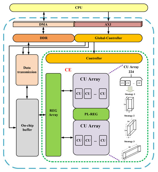
In order to solve the problem of heavy computational workload, which limits the deployment of deep convolutional neural networks on embedded devices, the hardware structure shown in Figure 13 was designed in [116]. In this hardware architecture, all buffers use the ping-pong data transfer mechanism to mask the data transfer time with the computation time to improve the performance.

Figure 13. Accelerator architecture based on a high-speed computing engine (CE) [116].

The computing engine (CE) is mainly composed of two computing unit (CU) arrays and several register arrays. Inside each computing unit is a “tree” structure of the bottom multiplier combined with the multilayer adder. Each CU array has 224 CU and can be configured to compute, in parallel, three different parallel modes of output feature maps of the dimension 4 × 14 × 4, 16 × 14 × 1, or 32 × 7 × 1. The flexible configuration ensures high CU utilization in different convolution parameters, so as to maintain a high operation speed. The register array includes the input feature map register (I-REG), the weight register (W-REG), the partial sum register (PS-REG), the output feature map register (O-REG), and the pooling register (PL-REG). On-chip buffers include buffers for input feature map (IBUF), weight (WBUF), partial sum (PBUF), and output feature map (OBUF). Each buffer consists of multiple blocks of RAM, which allow more data to be read or written simultaneously to improve read/write efficiency.

In this framework, the image and weight data were first added to the double data rate SDRAM (DDR) by the CPU-controlled direct memory access (DMA), and the top controller of the accelerator was configured, through which the control instructions were assigned to each module. The data transfer module reads the input data and weight parameters from the DDR to the on-chip buffer. Then, the computing engine (CE) performs the convolution operation, and the final result is written back to the DDR through the data transmission module. The architecture successfully deployed VGG-16, ResNet50, and YOLOv2-Tiny lightweight networks on a Xilinx ZynQ-7 ZC706 evaluation version operating at 200 MHz. The performances of 163 GOPS and 0.36 GOPS/DSP were achieved on VGG-16 with only 448 DSP resources.

Although this structure design achieves better performance and less resource consumption, on the whole, this structure does not consider the model parameter optimization of the fully connected layer, and the transmission overhead incurred when processing a large amount of data may limit the actual performance. In addition, this “tree” structure of a computing unit array can only process regular convolution operations. Although it can be configured into three different parallel modes in order to enhance the adaptability of the convolution layer to a certain extent, it is still not suitable for the convolutional neural network after sparse processing. Therefore, with the application of increasingly more irregular convolution operations, the usage scenarios of this hardware structure may be limited.

5.1.2. The RNN Accelerator Based on FPGA

Because the traditional RNN has the problem of gradient disappearance and explosion, the network performance is not good in the application, requiring long-term input information. Some researchers proposed a variant of RNN, long short-term memory (LSTM), to solve this problem. Although LSTM can solve the gradient disappearance problem, it cannot avoid the gradient explosion problem, and because it introduces many gating units, it leads to the problem of a large number of parameters [126]. Others have proposed the gate recurrent unit (GRU), which, like LSTM, has been put forward to solve problems such as long-term memory and gradients in back propagation [127]. In many cases, the GRU and LSTM are practically similar in performance. The largest difference between GRU and LSTM is that GRU combines the forgetting gate and the input gate into one “update gate,” and the network does not provide additional memory states. Instead, the output results are continuously recycled back as memory states, and the input and output of the network become particularly simple. However, GRU still cannot completely solve the problem of vanishing gradient.

In order to reduce RNN memory overhead for acoustic task, the [101] used a quantitative method to reduce the activation volume, wherein the time-consuming floating-point arithmetic was replaced by the faster floating-point arithmetic, greatly improving the network operation speed and joining the parameters of the mechanism of sharing and pipelined design in order to increase parallelism and reduce storage, further improving the network throughput and reducing the delay. However, the data quantized by this scheme is still the floating point. Fixed-point quantization can greatly improve the speed of data operation and reduce the memory overhead without much impact on the accuracy. Due to the feedback dependence of LSTM, high parallelism cannot be achieved on general processors such as the CPU and GPU.

The accelerator architecture firstly divides the input matrix and weight matrix into small blocks in advance, increases the parallelism of the matrix operation, and combines the pulsating array algorithm in order to accelerate the computation. Moreover, the problem of low data reading efficiency caused by data discontinuity during sequential data reading is solved by rearranging the elements in the matrix. Among them, the traditional processing element (PE) from memory read data performs various calculations and then writes the results back to the storage architecture, wherein the pulsating array appears in the form of lines, and each PE calculation no longer relies on memory access, only the first array PE in terms of reading data from memory, after processing the results directly to the next PE.

There are also some studies devoted to the compression of neural networks. Reference [129] proposed a hybrid iterative compression algorithm (HIC) for LSTM/GRU to compress LSTM/GRU networks. The utilization of block RAM (BRAM) is improved by rearranging the weights of the data stream of the matrix operation unit based on block structure matrix (MOU-S) and by fine-grained parallel configuration of matrix vector multiplication (MVM). At the same time, the combination of quantization and pruning greatly reduces the storage pressure.

5.1.3. The GAN Accelerator Based on FPGA

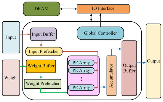
GANs mainly consist of a generator and a discriminator, producing better output through mutual game learning between generator G and discriminator D. In the original GAN theory, both G and D are not required to be neural networks, as long as the corresponding functions that are generated and discriminated against can be fitted. However, in practical application, deep neural networks used as G and D generally, so in the GAN accelerator design based on FPGA, it is basically aimed at the generator and the discriminator to optimize. Therefore, it is essentially optimized for CNN, RNN, or other neural network, mainly from the lower network number, wherein the accelerators are designed from the perspectives of reducing storage pressure, reducing computational complexity, and improving network computing speed.

The acceleration framework is shown in Figure 16. Firstly, the cascade fast FIR (finite impulse response) algorithm (CFFA) is optimized for GAN training, and the fast convolution processing element (FCPE) based on the optimization algorithm is introduced to support various computing modes during GAN training. In the input prefetcher module and weight prefetcher module, 16-bit fixed point and 8-bit fixed point were used, respectively, to process data, greatly improving the data processing speed. Finally, the architecture achieved 315.18 GOPS performance and 83.87 GOPS/W energy efficiency on the Xilinx VCU108 FPGA platform with 200 MHz operating frequency. Experiments showed that the architecture was able to achieve high energy efficiency with less FPGA resources. Although the architecture can effectively avoid the large consumption of hardware resources by cascading small parallel FIR structures to larger parallel FIR structures, this operation greatly increases the delay. When the number of cascades reaches a certain limit, the performance loss caused by the delay is incalculable.

Figure 16. The GAN acceleration framework.

5.2. Accelerator Design for Specific Application Scenarios

In the practical application of neural networks, people often customize FPGA accelerators with required functions according to specific application scenarios. Since accelerators customized according to specific application scenarios are relatively easy to design and can effectively solve the corresponding problems, this method is commonly used to accelerate neural networks in specific application scenarios, especially in speech recognition, image processing, natural language processing, and other fields.

5.2.1. FPGA Accelerator for Speech Recognition

Speech recognition is a technology that enables machines to automatically recognize and understand human spoken language through speech signal processing and pattern recognition. In short, it is the technology that allows a machine to transform a speech signal into a corresponding text or command through the process of recognition and understanding. Speech recognition has been applied in many fields, including speech recognition translation, voice paging and answering platforms, independent advertising platforms, and intelligent customer service. Speech recognition has strong real-time performance and high delay requirements, and thus it generally relies on the FPGA platform.

In terms of accelerating the application of speech recognition, the authors of [143] focused on the preprocessing stage of speech signals and proposed the use of a GAN to enhance speech signals and reduce noise in speech signals, so as to improve speech quality and facilitate speech recognition and processing. 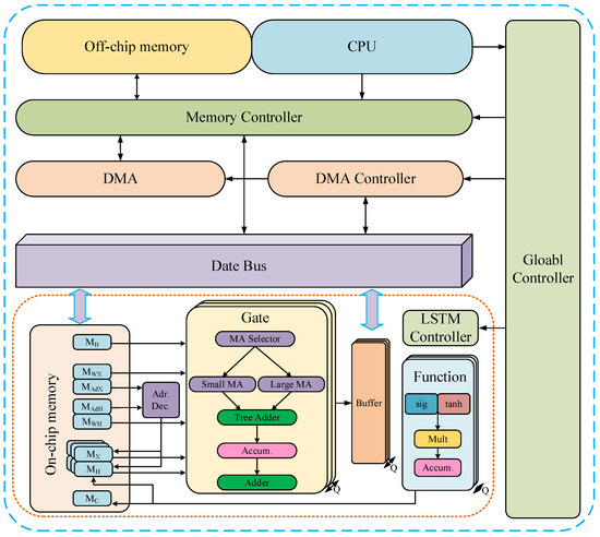In order to reduce energy consumption and improve the speed of speech recognition, the authors of [138] proposed an FPGA accelerator structure called balanced row dual-ratio sparsity inducing pruning algorithm (BRDS) for speech recognition, as shown in Figure 17. The accelerator compresses the LSTM network by pruning algorithm in order to reduce computational complexity and uses data reuse and pipeline design to achieve low power consumption and low delay. However, the acceleration architecture does not consider the problem of multi-core parallel load imbalance after LSTM model compression, which may occur in the actual use, thus affecting the performance of the whole accelerator.

Figure 17. BRDS: FPGA accelerator for speech recognition.

5.2.2. FPGA Accelerator for Speech Recognition

Image processing refers to the process of extracting, analyzing, and processing image information by computer, which is one of the earliest application fields of deep learning. Image processing techniques include point processing, group processing, geometric processing, and frame processing. The main research contents include image enhancement, image restoration, image recognition, image coding, image segmentation, among others. Since 2012, ImageNet competition, image recognition, and processing technology have been widely used in image classification, face recognition, and other fields. In the design of an FPGA accelerator for image processing, the accelerator is designed mainly for the purpose of reducing the amount of data, memory, and computation demand [97,144,145,146].

5.2.3. FPGA Accelerator for Natural Language Processing

Natural language processing (NLP) is a technology that uses the natural language used by humans to communicate with machines. It studies various theories and methods that can realize effective communication between humans and computers using natural language, and it is also one of the important application fields of deep learning.

在加速NLP方面，[152]的作者指出，尽管基于转换器[153]的语言表示在各种NLP任务上已经达到了最先进的精度，但大型模型网络的部署一直是资源受限计算平台的挑战。权重修剪用于减少权重参数，可以有效压缩网络模型，提高网络性能。为了解决将RNN应用于自然语言处理时，大量参数导致的存储需求大和网络性能下降的问题，[154]的作者针对RNN的计算资源需求，采用定点量化技术设计了FPGA加速器，减少了90%的内存消耗。并且精度损失小于1%。

5.3. 用于优化策略的 FPGA 加速器

在基于FPGA的神经网络加速器设计中，往往需要研究神经网络的特性，并根据其运行特性进行有针对性的优化，其中合理的优化策略可以显著提高加速器的性能和资源利用率，这是优化计算的常用优化策略，和存储优化，以及其他改进。

5.3.1. 计算优化

在神经网络中，卷积层和卷积操作通常是重点，尤其是在应用于图像处理的卷积神经网络中。卷积操作更密集，处理时间更长，资源占用更多，这限制了卷积神经网络在FPGA等边缘平台中的部署。

通常的优化方向是增加神经网络模型不同层之间的并行度、不同输出特征图之间的并行度、不同像素之间的并行度、不同像素之间的并行度，以缩短处理时间，提高网络性能。它还可以使用循环流和循环展开来构建更深层次的管道，以缩短网络的整体执行时间并减少时间开销。矩阵周期通过循环块技术划分为更小的模块，每个模块可以并行计算，以提高计算并行性。

5.3.2. 存储优化

由于神经网络中的数据和参数量很大，在部署神经网络时，参数和数据存储的问题不可避免。在存储的优化中，通常采用降低数据精度的策略来减少数据量，从而提高操作速度。可以采用数据复用方法，以大大减少数据存储和内存空间占用。

5.4. 其他 FPGA 加速器设计

除了上述加速器设计外，还有其他一些加速器设计，例如基于硬件模板的加速器设计。通过使用现成的硬件模板来设计加速器，只需要根据具体问题对模块进行改进和配置参数，这大大提高了模型的部署[162]。

This entry is adapted from the peer-reviewed paper 10.3390/app122110771

© Text is available under the terms and conditions of the Creative Commons Attribution (CC BY) license; additional terms may apply. By using this site, you agree to the Terms and Conditions and Privacy Policy.