Your browser does not fully support modern features. Please upgrade for a smoother experience.
Please note this is an old version of this entry, which may differ significantly from the current revision.
Subjects:
Optics
Inspired by the fast development of deep learning, people have combined the DL techniques with inverse design. At present, DL has been developed rapidly in the field of photonic device inverse design, which can be more efficient than traditional iterative optimization methods.
- photonics
- inverse design
- deep learning
- adjoint method
1. DL Networks Applied to Photonic Inverse Design
Deep neural networks are often built on top of fully connected networks (FCNs) and convolutional neural networks (CNNs). FCNs can be viewed as the most primitive type of neural networks, which are composed of multiple layers of neurons, each being connected to all other ones on the adjacent layer. The fully connected nature offers FCNs the ability to simulate complex transformations. The computation between two adjacent layers can be mathematically described by a matrix–vector product or its tensor counterpart. Suppose that the number of neurons is N for the two adjacent layers, and the computational complexity of the associated layers reaches 𝑂(𝑁2). The high complexity prevents FCN in practice from having a large number of layers and neurons. CNNs are an improved alternative to FCNs where the time-consuming matrix–vector operations (or its tensor counterpart) are replaced with the convolution operations. The invariance of the translation of the input tensor in CNNs enhances the ability of the networks to capture features from image/audio data with strong spatial/temporal correlation. When it comes to sequential data, recurrent neural networks (RNNs) [95] become the most commonly used models, which can be unambiguously generalized to sequentially connected neurons.
1.1. Fully Connected Networks (FCNs)
In [92], the plasmonic waveguide-coupled with cavities structure (PWCCS) was optimized by employing a FCN, as shown in Figure 1. The effectiveness of the FCN in optimizing the PWCCS was verified via the selection of Fano resonance derived from PWCCS and plasmon-induced transparency effects. In this work, the genetic algorithm was employed to design network structures and to guide the selection of hyperparameters for the FCN. Such an approach not only enables the high-precision inverse design of PWCCS but also optimizes some key performance indicators of the transmission spectrum. In [96], the inverse design of the edge state of the curved wave topology was realized via FCNs. In this work, two neural networks were constructed for the forward and backward predictions of bandgap width and geometric parameters. The dataset used to train a feed-forward artificial neural network was generated using the plane wave expansion method (PWE) with a sweeping of the arrangement radii.
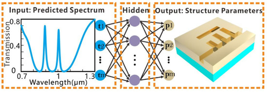
Figure 1. Diagram of the ANNs applied in the inverse design and performance optimization problems [92].
1.2. Convolutional Neural Networks (CNNs)
As it is known, CNNs can capture the local correlation of spatial information in the input data. This property is highly desired in photonics applications as the devices are always represented by high-dimensional spatial data. Consequently, CNNs and their improved variations have attracted many researchers who applied them to the solution of inverse design problems. For example, it has been proved that CNNs had the potential to solve the problem of the inverse design of thin film metamaterials, probing the parameter space of a given material and thickness library globally, which can be difficult and expensive for traditional methods [97]. The full generalization ability of neural networks, especially CNNs, to generate systems with the desired spectral response to accommodate various input design parameters has been revealed.
In [98], the CNN was employed to be an inverse design tool to achieve high numerical accuracy in plasma element surfaces, which proved that the CNN was an excellent tool for the design. More specifically, the CNNs are capable of identifying peaks and troughs of the spectrum at the expense of low computational cost. Key geometric parameters can reach an accuracy as high as ±8 nm. In this work, the comparison of CNNs and FCNs shows that CNNs had higher generalization capabilities. Additionally, it has been demonstrated that batch normalization can improve the performance of CNNs.
1.3. Recurrent Neural Networks (RNNs)
RNNs tackle problems associated with sequential data such as sentences and audio signals. The network receives sequential data one at a time and incrementally generates new data series. It was demonstrated in [99] that, for photonic design, RNNs were suitable to model optical signals or spectra in the time domain with a specific line shape originating from various modes of resonance. In [100], RNNs were implemented to analyze optical signals and to equalize noise in high-speed fiber transmission. In [77], RNNs were utilized to find the correlation within 2D cross-sectional images of plasmonic structures, where the results showed that the network was able to predict the absorption spectra from the given input structural images. It was revealed in [101] that the performance of RNNs can be enhanced by adopting advanced varieties of RNNs, such as Long Short-Term Memory (LSTM) [102] and gated recurrent unit (GRU). In [103], traditional neural networks, RNNs with LSTM and an RNN with GRU were used to construct the inverse design of MPF. As indicated by the results in [103], according to the training results, it was found that GRU-based RNNs were the most effective in predicting frequency response with the highest accuracy. The study in [104] demonstrated that, in combination with CNNs, RNNs were also utilized to enhance the approximation of the optical responses of nanostructures that are illustrated in images. As revealed in [99], network systems hybridizing CNNs and RNNs present a promising method for modeling and designing photonic devices with unconventional spatiotemporal properties of light.
1.4. Deep Neural Networks (DNNs)
A DNN is a network where the number of hidden layers is much greater than 1. The DNNs can be divided into discriminant neural networks and generative ones. In this subsection, we focus on the discriminant DNNs and delay the discussion on the generative ones in the following Section 3.1.5.
As pointed out in [105], neural networks can be used in two different ways. The first method takes the configuration of the device to be designed including the structural parameter (such as the geometrical shape of a nanostructure) as the input and the predicted electromagnetic response of the device (such as transmission spectra or differential scattering cross-section) as the output. These neural networks can be used to replace the computationally expensive electromagnetic simulations in the optimization loop, greatly reducing the design time. In [105], the DNNs belonging to this method were denoted by forward-modeling networks because they compute electromagnetic response from the device. Essentially, a forward-modeling DNN is an electromagnetic solver. The second type of neural network, named after inverse-design networks, takes the electromagnetic response as the input and directly outputs the configuration of the device. The inverse-design networks act as an inverse operator that converts the electromagnetic response to the configuration of the device. However, one significant difficulty in training inverse-design DNNs arises from a fundamental property of the inverse scattering problem: the same electromagnetic response can be produced using many different designs. Different from the previous remedy to this difficulty where the training dataset was divided into distinct groups, where there was a unique design within each group corresponding to each response, the approach of cascading an inverse-design network with forward modeling was proposed in [105]. The obtained network was named the tandem DNN. Numerical experiments in [105] indicated that the tandem DNNs can be trained by datasets containing nonunique electromagnetic scattering instances.
In [93], the so-called iterative DNN was proposed, where trained weights of the forward modeling network [105] were fixed and gradient-descent methods based on backpropagation were employed. The iterative DNN and tandem DNNs were compared in terms of the transmission spectrum design of bow nanoantennas, where the results demonstrated that the two types of DNN architectures reached comparable performance.
In [106], three models were investigated for designing nanophotonic power splitters with multiple splitting ratios. The first model employed the DNN as a forward-modeling network to predict the spectral response (SPEC) given hole vectors (HV). The second one utilized the DNN as an inverse-design network to construct HV given a target SPEC. The third one was based on a stochastic generative model which implicitly integrated forward and inverse-design networks. In addition, a bidirectional network consisting of the forward and inverse-design networks was proposed [107]. The forward-modeling network was trained subsequently to the inverse-design network, which was used to predict the geometry from the transmission spectrum.
In [108], DNN models were used as both the electromagnetic solvers and the optimizer. By building the DNN with an FDTD solver, the proposed method can be used to efficiently design a silicon photonic grating coupler, one of the fundamental silicon photonic devices with a wavelength-sensitive optical response.
To facilitate multi-tasks inverse design, a topology optimization method based on the DNN in the low-dimensional Fourier domain was proposed in [109]. The DNN took target optical responses as inputs and predicted low-frequency Fourier components, which were then utilized to reconstruct device geometries. By removing high-frequency components for reduced design degrees of freedom (DoFs), the minimal features were controlled and the training was sped up. In [110], a forward-modeling DNN was paired with evolutionary algorithms, where the DNN was used only for preselection and initialization. The method utilizes a global evolutionary search within the forward model space and leverages the huge parallelism of modern GPUs for fast inversion.
A well-organized tutorial was given in [111], where the process of deep inverse learning applied to AEM problems was given in a step-by-step approach. In [111], common pitfalls of training and evaluation of DL models were discussed and a case study of the inverse design of a GaSb thermophotovoltaic cell was given.
1.5. Deep Generative Models
Generative models generally seek to learn the statistical distribution of data samples rather than the mapping from input to output data. In this respect, they can be viewed as the complement techniques of the conventional optimization and inverse design [35]. In generative models, the joint distribution of the input and output is employed to optimize a certain objective in a probabilistically generative manner instead of determining the conditional distribution and thus decision boundaries.
Generative adversarial networks (GANs) are the typical deep generative models built using generators and discriminators, which have been used for the design and optimization of dielectric and metallic metasurfaces due to their ability to generate massive nanostructures efficiently [112,113].
In [114], a conditional deep CGAN was employed as an inverse-design network, which was trained on colored images encoded with a range of material and structural parameters. It was demonstrated that, in response to target absorption spectra, the CGAN can identify an effective metasurface in terms of its class, material properties, and overall shape. In [115], a meta-heuristic optimization framework, along with a resistant autoencoder (AE), was designed and demonstrated to greatly improve the optimization search efficiency for meta-device configurations featuring complex topologies.
In [36], a network combining the CGAN with the WGAN was proposed to design free-form, all-dielectric metasurface devices. This work indicated that the proposed approach stabilized the training process and gave the network the ability to handle synthetic metasurface design problems. It also demonstrated in this work that GAN-based approaches were the preferred solution to multifunctional inverse design problems.
In [12], research was conducted on inverse models that utilize unsupervised generative neural networks to exploit the benefits of not requiring training data samples. However, time-consuming electromagnetic solvers must be integrated into the generative neural networks to guarantee compliance with the laws of physics. After training, unsupervised generative neural networks can also generate new geometric parameters based on the optical response of the target without the need for any electromagnetic solver [12].
2. Limitations of DL in Photon Inverse Design
Although DL is attractive in inverse design photonics, there are still limitations with DL algorithms. These limitations include the DoFs, the local minimum, the difficulty in preparing the DL training dataset, the nonunique solutions, and difficulties associated with generalization.
2.1. Degrees of Freedom
In topological optimization, the number of DoFs can be very large, which always makes the DL very hard to train. The relationship between geometric parameters and optical performance is very similar to the mathematical non-deterministic polynomial difficulty (NP difficulty) problem [116] and very hard to define using explicit functions. As shown in Figure 2 from [12], the designer extracts the geometric parameter x from a device structure, such as an empirical structure, the QR code one, or an irregular one.
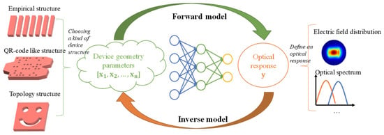
Figure 2. Schematic of DNN-assisted silicon photonic device design approach [12].
What ML method can be employed in inverse design is related to the DoFs of the photonic structure. For the case with a relatively small number DoFs, many DL networks can be employed in the inverse design. However, the DoFs continue to grow to thousands or more, and the huge dimension of the optimization space prohibits methods that require large amounts of data or a lot of simulation iterations. In this case, the generative models, such as GANs and VAEs, can be leveraged to reduce the dimensionality of the design structure and optical response [33,117].
Additionally, the DoFs of photonic devices could potentially impact the NLO phenomenon. For example, due to the varying interlayer interactions associated with different twist angles, the twisting DoFs have been widely applied to engineer the bands of van der Waals layered structures. In that work, the twist-angle-dependent second-harmonic generation (SHG) from twisted bilayer graphene samples was demonstrated along with their correlation with the evolving hybrid band structure [118]. Nonlinear optics will probably be increasingly important since people can reach a better understanding of the underlying physics although the design involves many DOFs, i.e., many photonic DOFs, such as spatial modes, frequencies, and polarizations, and many design parameters, such as the space- and time-dependent distributions of refractive index and loss/gain in photonic structures [119]. Furthermore, reconfigurable control of many modal DOFs can be achieved with spatial light modulators or digital micromirror devices, which are now available with resolutions (i.e., number of pixels) close to 107107 [119]. In general, the number of design DOFs routinely available to optical scientists and engineers now exceeds the technology from past decades by 3 to 5 orders of magnitude [119].
2.2. Training Dataset
DL often requires large and high-quality training datasets, which are generally unavailable in practice. The large amount of data required for DL could not be readily available and is usually created using simulation methods such as RCWA, FEM, and FDTD, which are time- and computation-expensive [33,90,120]. In [35], a dataset of 20,000 two-dimensional photonic crystal unit cells and their associated band structures was built, enabling the training of supervised learning models. Using these datasets, a high-accuracy CNN for band structure prediction was demonstrated, with orders-of-magnitude speedup compared with conventional theory-driven solvers. In [107], a DNN was trained using a dataset composed of 15,000 randomly generated device layouts containing eight geometrical parameters. In [121], to train a forward network model for prediction of electromagnetic response, a dataset of 90,000 samples was generated using 𝑆4 software (version 2) [122], where the lattice constant was set between 50 nm and 150 nm and the maximum thickness of each dielectric was limited to 150 nm.
An effective way is to co-construct large datasets of various optical designs with the efforts of the optical community [33,123] by avoiding the repeated generation of simulation data. To use generative models instead of real datasets is also a nice alternative [32]. Another solution is to develop networks suitable for small training datasets. In [27], an approach based on explainable artificial intelligence was developed for the inverse design, demonstrating that their method works equally well on smaller datasets. In [124], an efficient tandem neural network with a backpropagation optimization strategy was developed to design one-dimensional photonic crystals with specific bandgaps using a small dataset.
In [125], methods to generate datasets with high quality were discussed to overcome the problem arising from the lack of training data. The optimization algorithm in [126] to generate training data may perform less efficiently as it is time-consuming for the case of many free parameters. The concept of iterative training data generation has emerged as the remedy, which allows the neural network to learn from previous mistakes and to significantly improve its performance on specific design tasks. However, iterative procedures can be computationally expensive since data generation is slow and the network may need to be re-trained several times on increasing amounts of training samples [115]. The solution is to reduce the amount of re-training by accelerating convergence by assessing the quality and uncertainty of the ANN output from multiple predictions. In addition, transfer learning has also been applied in nano-optics problems to enhance the performance of the ANN when the available data are limited [127].
2.3. Nonuniqueness Problem
Since different designs may produce almost identical spectra, this may prevent ML algorithms from converging correctly. Many researchers have developed various solutions to this problem. In [77,121], a method adding forward modeling networks to the inverse design DNN architecture was employed, which can be viewed as one of the most common ways to overcome the nonunique problem. In [128], an approach modeling the design parameters as multimodal probability distributions rather than discrete values was proposed, which can also overcome the nonunique problems. In [129], a physics-based preprocessing step to solve the size mismatch problem and to improve spectral generalizability was proposed. Numerical experiments in this work indicated that the proposed approach can provide accurate prediction capabilities outside the training spectrum. In [124], an algorithm called adaptive batch normalization was proposed, which was a simple and effective method that accelerates the convergence speed of many neural networks.
2.4. Local Minimum
Similar to the AM, DL also to some extent relies on gradient information to carry out the optimization. Thus, DL inverse design can also suffer from local minimum problems. In [130], an approach to overcome the local minimum problem was proposed by constructing a combined loss function that also fits the Fourier representation of the target function. Physically, the Fourier representation contains information about the target function’s oscillatory behavior, which corresponds directly to specific parameters in the input space for many resonant photonic components. In [33], the generative models were incorporated into traditional optimization algorithms to help avoid local minimum problems. Because generative models are essentially transforming raw data into another representation, the local minimum problem in the original parameter space may be eliminated, which can alleviate the local minimum problem if optimized in a sparse representation. In [131], deep generative neural networks based on global optimization networks (GLOnets) were configured to perform categorical global optimization of photonic devices. This work showed that, compared with traditional algorithms, GLOnets can find the global optimal several orders of magnitude faster.
2.5. Generalization Ability
The lack of generalization can also limit DL in inverse design [132]. DL is like a black box, making it challenging to understand and interpret its results and reliability, especially when dealing with imperfect datasets or data generated by adversarial methods. Due to the challenges of validating and replicating DL results, a set of community-wide recommendations in biology for DL reporting and validation (data, optimization, model, and evaluation) was recently published. The given recommendations help to handle questions that need to be addressed when reporting DL results and are also largely applicable to the fields of optics and photonics [91].
2.6. Problem of Rerunning
When the optimization goal is modified, a new inverse optimization process needs to be rerun, maybe from scratch. Since a single run of traditional inverse design optimization is always time- and computation-expensive as it may require hundreds of rounds of simulations, rerunning will consume a large amount of computing resources [77]. Moreover, when the optimization goal is modified, it is necessary to recreate the dataset if DL is employed, which is large in amount and not readily available. In the AM, the change of optimization goal requires additional derivation steps for different cases, leading to extra work when switching parameterizations [70].
This entry is adapted from the peer-reviewed paper 10.3390/photonics10070852
This entry is offline, you can click here to edit this entry!