Your browser does not fully support modern features. Please upgrade for a smoother experience.
Please note this is an old version of this entry, which may differ significantly from the current revision.
An improved YOLOv5 model is used to detect vehicles in aerial images in this paper, which effectively enhances the detection performance of tiny objects and obscured vehicles.
- vehicle detection
- UAV imagery
- YOLOv5
- Feature Fusion Network
- Soft-NMS
1. Introduction
The usage of small, low-altitude UAVs has snowballed in recent years [1,2,3,4]. Objection detection techniques based on UAVs equipped with vision sensors have attracted much interest in areas such as unmanned vehicles and intelligent transportation systems [5,6,7,8]. UAV-based aerial vehicle detection techniques are less expensive than cameras installed at fixed locations and produce more extensive image views, greater flexibility, and broader coverage. UAVs can monitor road traffic over any range and provide critical information for subsequent intelligent traffic supervision tasks such as traffic flow calculation, unexpected accident detection, and traffic situational awareness. However, the vast percentage of vehicle targets have few feature points and small sizes [9,10], which presents a difficulty for precise and real-time vehicle detection in the UAV overhead view [11].
Existing vehicle detection approaches can be roughly divided into traditional and deep learning-based vehicle detection algorithms. Traditional vehicle detection algorithms must extract features [12,13] manually and then use SVM, AdaBoost, and other machine learning methods for classification. However, this way is time-consuming and can only extract shallow features, which has significant limitations when applied to aerial photography scenes with small targets. In recent years, with the continuous development of deep learning techniques, various artificial intelligence algorithms based on convolutional neural networks have played a great role in different fields, such as autonomous driving [14], optimization of medicine policies [15], and wildlife census [16]. Deep learning-based target detection algorithms have also been extensively applied, mainly including two-stage and single-stage algorithms. Two-stage target detection algorithms need to extract candidate regions first and then perform regression localization and classification of targets, with common examples including: Fast R-CNN [17], Faster R-CNN [18], and R-FCN [19]. Singh et al. [20] used Fast R-CNN-optimized samples to design a real-time intelligent framework that performs well on vehicle detection tasks with complex backgrounds and many small targets. Nevertheless, the model may not fit well for cases where the objective sizes vary widely. The authors of [21] conducted a study on vehicle detection based on Faster R-CNN, and the improved model reduced the latency and enhanced the detection performance for small targets. However, the model requires high computational resources in the detection process. Kong et al. [22] use a parallel RPN network combined with a density-based sample assigner to improve the detection of vehicle-dense areas in aerial images. However, the model structure is complex and requires two stages to complete the detection, which cannot meet the requirement of real-time detection. Since the two-stage detection algorithm requires the pre-generation of many pre-selected boxes, it is highly accurate but slow and cannot meet the needs of real-time detection [23]. The single-stage target detection algorithm directly transforms the localization and classification problem into a regression problem, which has an absolute speed advantage and accuracy potential compared with the two-stage one. The mainstream single-stage target detection algorithms mainly include the YOLO (You Only Look Once) series [24,25,26,27] and the SSD series [28]. Yin et al. [29] obtained outstanding detection performance for small objects by improving the efficiency of SSD in using feature information at different scales. However, the default box needs to be selected manually, which may affect the performance of the model in detecting small targets. Lin et al. [30] detect oriented vehicles in aerial images based on YOLOv4, and the improved model significantly improved the detection performance in scenarios with densely arranged vehicles and buildings. However, further improvement studies are lacking for scenes with small targets. Adel et al. [31] compared the detection performance of Faster R-CNN, YOLOv3, and YOLOv4 on the UAV aerial vehicle dataset but without considering the impact of vehicle occlusion, shooting angle, and lighting conditions on the model. Zhang et al. [32] propose a novel multi-scale adversarial network for improved vehicle detection in UAV imagery. The model performs great in images from different perspectives, heights, and imaging situations. However, the classification of vehicles is not specific enough, with only two categories: large vehicles and small vehicles.
Because of its excellent detection accuracy and quick inference, YOLOv5 [33] is applied extensively in various fields for practical applications. Niu et al. [34] used the ZrroDCE low-light enhancement algorithm to optimize the dataset and combined it with YOLOv5 and AlexNet for traffic light detection. Sun et al. [35] employed YOLOv5 to identify the marks added to bolts and nuts, from which the relative rotation angle was calculated to determine whether the bolts were loose. Yan et al. [36] applied an enhanced model based on YOLOv5 to apple detection, which improved the detection speed and reduced the false detection rate of obscured targets.
2. Real-Time Vehicle Detection Based on YOLOv5
2.1. Overview of YOLOv5
YOLOv5 is a single-stage target detection algorithm released by Ultralytics in 2020 that consists of four structures: YOLOv5s, YOLOv51, YOLOv5m, and YOLOv5x. The model works by dividing the image into multiple grids, and if the center of the target falls within a grid, that grid is responsible for predicting the object. YOLOv5s is the most miniature model in depth and width among these four models. With the increase in model size, although the detection accuracy improves, the detection speed also becomes slower. As shown in Figure 1, YOLOv5s network is mainly categorized into four parts: input layer(input), backbone, neck, and prediction layer (head).
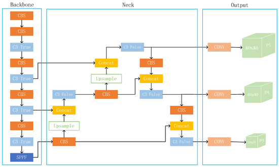
Figure 1. The framework of the YOLOv5s algorithm.
The primary function of the input layer is to unify the size of the input image into a fixed size. The backbone section, which includes the CBS, C3, and SPPF modules, is primarily responsible for extracting essential information from the input picture. The structure of each module is shown in Figure 2. The Neck portion of YOLOv5 employs a mixed structure of FPN [39] and PAN [40]. FPN transfers semantic information from deep to shallow feature maps, while PAN conveys localization information from shallow to deep feature layers. The combination of the two may aggregate characteristics from multiple backbone levels to different detection layers, enhancing the feature fusion capacity of the network.
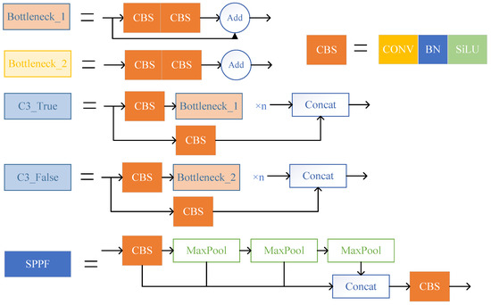
Figure 2. Structure diagram of CBS, C3, and SPPF modules.
2.2. Adding a Prediction Layer for Tiny Objects
The maximum downsampling step of the YOLOv5s network is 32. Therefore, a resolution less than 32 × 32 pixels is regarded as a small target [41], greater than 96 × 96 pixels is defined as a large target, and in between is classified as a medium target. Since there are a large number of targets with tiny scales in the pictures taken by UAVs, scholars further subdivide the targets with a resolution less than 32 × 32 pixels into two cases of tiny (resolution < 16 × l6 pixels) and small (16 × 16 pixels < resolution < 32 × 32 pixels). The obtained target scale distribution is shown in Figure 3. It can be found that the number of tiny objects in train, val, and test are all significant. Therefore, it is essential to customize a detection layer more suitable for detecting tiny targets.
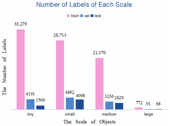
Figure 3. Number of objects at different scales in this dataset.
The YOLOv5s network has three detection layers, P3, P4, and P5, with feature map sizes of 80 × 80, 40 × 40, and 20 × 20, respectively. The larger size of the feature map is responsible for detecting smaller objects. The largest 80 × 80 feature map corresponds to an input size of 640 × 640, and the receptive field size of a grid in the feature map is 8 × 8. If the height or width of a tiny vehicle in the original image is less than 8 pixels, it is difficult for the network to learn the features of the object. The new P2 detection branch can detect targets at the 4 × 4 pixel level while configuring anchor boxes of smaller size, thus effectively reducing the missed detection of tiny vehicles.
From Figure 4, it can see that the first C3 module in the Backbone outputs a feature map of 160 × 160 after two downsamplings, while the second C3 module produces a size of 80 × 80. The scholars fuse the feature map of 160 × 160 with the output of the second C3 module after upsampling to obtain the detection branch P2. In this way, the input of P2 derives mainly from the shallow convolutional layer and contains more information related to shape, position, and size. This information facilitates the model to discriminate fine-grained features more accurately, thus improving the capability to detect small targets.
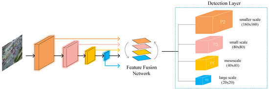
Figure 4. YOLOv5s algorithm framework with the added tiny object detection layer.
2.3. Enhancing Feature Fusion with Bifpn
The Neck part of YOLOv5 uses a combined FPN and PAN structure. When it comes to feature extraction, the shallow network has a higher resolution and more precise position information. On the other hand, the deeper network has a more extensive receptive field and more high-dimensional semantic information that aids with object categorization. FPN facilitates semantic information from deep feature maps to shallow feature maps, while PAN accomplishes a high degree of integration between shallow localization information and deep semantic information. The combination of FPN and PAN, which aggregates parameters from multiple backbone levels to distinct detection layers, significantly improves the feature fusion capabilities of the network.
Nevertheless, there is a problem in that input to the PAN structure is largely feature information processed by FPN, with no original feature information taken from the backbone network. This issue may cause the optimization direction of the model to be biased, affecting the detection impact. The BiFPN first simplifies the PAN structure by removing the nodes with only one input and output edge. Then, an extra edge is added between two nodes at the same level to fuse more differentiated features, and the structure is shown in Figure 5C. The original BiFPN would assign various weights to different input features according to their importance, and this structure is utilized frequently to encourage feature fusion. The introduction of BiFPN with weights, however, increases the number of parameters and calculations for the dataset in this research, and the detection effect is not satisfactory.
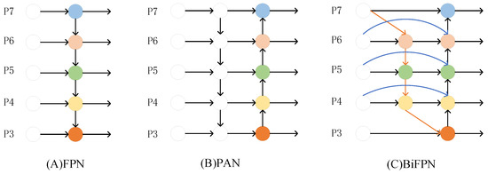
Figure 5. Schematic diagram of different feature fusion structures.
Because the motivation for introducing BiFPN is that PAN can obtain more original feature information as input, scholars remove the weighted part and only reference its cross-scale connection way. By introducing the de-weighted BiFPN, the trade-off between accuracy and efficiency is considered, making the feature fusion process more reasonable and efficient. In this way, each node of PAN has one input edge from the backbone network, making the training process have continuous involvement of the original features and preventing the model from deviating from the expectation during the training process. The feature information of tiny targets is already relatively insufficient, and the features are easily missing after several convolutions. As shown in Figure 6, part of the input of the added prediction layer is from the first C3 module. This module retains most of the original feature information. Thus, more features about the tiny objects can be obtained, and the detection performance of the model can be improved.
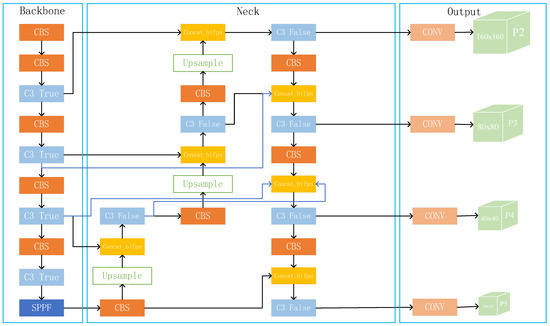
Figure 6. Network structure diagram after improving Neck and Head parts.
2.4. Introducing Soft-NMS to Decrease Missed Detections
The NMS algorithm selects the one with the highest confidence among all the predictor frames then conducts IoU operations sequentially with other predictor frames. For a prediction box whose IoU value exceeds the set threshold, it is directly deleted. During peak commuting hours, the vehicle density in the images captured by the UAV is high and closely aligned. In this circumstance, using the NMS algorithm suppresses many anchor frames that initially belonged to different targets, resulting in the missed detection of obscured vehicles.The NMS algorithm is shown in Equation (1).
where 𝑏𝑖 and 𝑠𝑖 denote the ith predictor box and its score, respectively, and 𝑁t is the set threshold. M indicates the candidate box with the highest score. When the IoU of M and 𝑏𝑖 is greater than the threshold, the score 𝑠𝑖
of b is directly set to 0, likely to erroneously remove some prediction boxes containing vehicles.
Unlike the NMS method, Soft-NMS selects M as the benchmark box then calculates the IoU between M and the neighboring predictor boxes. This adjacent prediction frame is not suppressed when the IoU value is less than the set threshold. When the IoU value is greater than the set threshold, the penalty function attenuates the scores of the prediction frames that overlap with the reference frame instead of directly setting the scores to 0. By penalizing the scores of prediction frames with large IoU values, anchor frames with larger overlap areas get higher penalty coefficients and more minor scores 𝑠𝑖
. Thus, there is a chance they are preserved during the suppression iterations, avoiding the situation where highly overlapping prediction frames contain targets but are removed.
The expression of the Soft-NMS algorithm is given in Equation (2).
where 𝜎 is the hyperparameter of the penalty function. Combining with Equation (2), it can be seen that when the overlap of two boxes is higher, the value of IoU(𝑀,𝑏𝑖)2 is larger and 𝑠𝑖

is smaller. So the predicted box obtains a smaller score but can be retained instead of directly deleted, thus avoiding the missed detection of overlapping vehicles.
Figure 7a compares the detection performance of YOLOv5 using NMS and Soft-NMS as prediction frame screening algorithms. By focusing on the red dashed box in Figure 7b, it can be found that the application of the Soft-NMS algorithm successfully decreases the number of missed vehicles in the densely arranged region and enhances the detection performance of the model in the high-overlap scenario.

Figure 7. Comparison of YOLOv5s algorithm detection results before and after using Soft-NMS. (a) The detection performance of YOLOv5; (b) The detection performance of YOLOv5 after the introduction of Soft-NMS.
This entry is adapted from the peer-reviewed paper 10.3390/s23125634
This entry is offline, you can click here to edit this entry!
