Artificial intelligence (AI) gives computers the ability to make decisions via analysing data independently, following predefined rules or pattern recognition models. In the field of biotechnology, AI is widely used for various research challenges, most notably for de novo protein design, where new proteins with envisaged functions are assembled using amino acid sequences not found naturally according to the physical principles underlying intra- and intermolecular interactions [61,62,63,64]; in protein engineering, where selected proteins are manipulated to tailor selected key properties, e.g., activity, selectivity and stability [61,65]. Here, AI has been particularly useful when used to assist directed evolution experiments, namely by enabling a reduction in the number of wet-lab iterations required to generate a protein with the intended features [61,66,67]. Additionally, AI has been used in the field of biopharmaceuticals (drugs and vaccines) to develop new drugs, redefine existing and marketed drugs, understand drugs’ mechanism and mode of operation, design and optimize clinical trials and identify biomarkers. AI is also used in the analysis of genomic interaction and the study of interaction pathways, protein-D, cancer diagnosis and analysis of genetics, among other applications [68,69,70]. Machine learning (ML) is a subfield of AI that allows the development of computer programs that learn and improve their performance automatically based on experience and without being explicitly programmed. In various studies, ML improvement strategies from large datasets generated by different techniques have been advantageously used for different purposes, such as the identification of weight-associated biomarkers [71], discovery of food identity markers [72], elucidation of animal metabolism [73] and investigation of many other areas of metabolomic development [74,75]. Many studies highlight the essential advantage of using ML and systems biology in pathway discovery and analysis, identifying enzymes, modelling metabolism and growth, genome annotation, the study of multiomics datasets, and 3D protein modelling [76]. Based on the available data, ML algorithms allow finding patterns, which represent points with several characteristics or descriptors, e.g., enzyme sequences, their secondary and tertiary structures, substitutions, physicochemical properties of amino acids, etc. These properties usually range from tens to thousands in number, and are thus hard and extremely time-consuming to handle using conventional approaches.

ML can be implemented through unsupervised and supervised learning. Unsupervised learning reduces high-dimensional data to a smaller number of dimensions or identifies patterns from data. In turn, in supervised learning, algorithms use data labelled in advance (designated as a training set) to learn how to classify new, testing data. Labelled data thus consist of a set of training examples, where each example is composed of an input and a sought-after output value. Thus, major features or combinations of features are obtained, and can henceforth improve the label accuracy in the training set and further use the gathered information for future input labelling. To put it another way, one or several target characteristics, e.g., enzyme activity, specificity or stability, can be designated as labels. The goal is to design a predictor that will return labels for unseen data points based on their descriptors using a properly tagged training dataset. Supervised and unsupervised methods can be combined under specific conditions to yield semi-supervised learning [77,78].

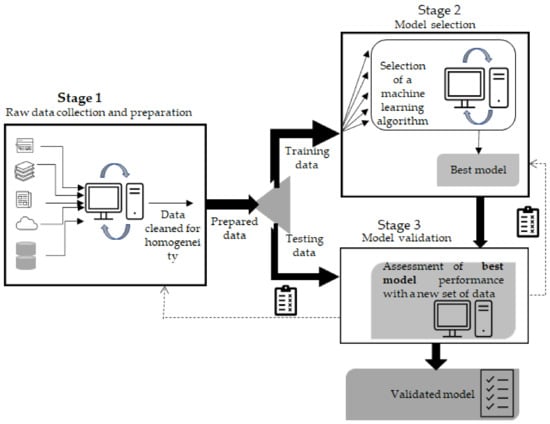
Supervised learning is by far the preferred approach in enzyme engineering, as the focus is on improving one or more properties of the enzyme [78]. Overall, the process flow of machine learning can be divided in three stages (Figure 1). Stage 1, which involves data collection, recording and preparation of the input to be fed to the algorithm, is often considered the most laborious phase. The databases BRENDA, EnzymeML, IntEnzyDB, PDB Protein Data Bank and UniProtKB (these and further examples given in [78,79,80,81]) are by far the preferred sources for acquiring information. However, to extract useful information from the retrieved dataset, the data must be adequately pre-processed or cleaned, e.g., managing errors and missing data, detecting and removing duplicates, outliers and irrelevant information, as the quality of data heavily influences the precision of the final outcome [82]. Within this scope, and with the aim to facilitate the use of information throughout multiple scientific areas, steps towards the standardization of data and of semantics have been recently achieved [83]. In stage 2, algorithms process the data that is to be fed to the selected model. The final stage involves model validation using test data. Between stages 1 and 2, the available experimental data are split into two parts: part of the data are used for training subsets and adjusting the parameters of a predictor (stage 2); the remaining data are diverted to stage 3 for the final evaluation [78,84]. The algorithm also has to learn how to classify input data, e.g., assign a label such as spam/not spam. In terms of classification steps with binary labels or labels with a finite number of options, this evaluation is usually based on the number of true confusion matrices: positive and negative true/false. Here, a confusion matrix can be described as a summary of prediction results for a classification problem [78,85]. Classification is evaluated based on the sensitivity and specificity of the results [77]. For the regression steps, where the relationship between independent variables or features and a continuous dependent variable or outcome is addressed, the quality of the prediction is typically evaluated using root mean square deviation [77,78]. The final assessment (stage 3) is carried out on the test dataset. This is paramount as the goal is to ensure the robustness of a model through its successful application to datasets other than those used for training. In enzyme engineering, the occurrence of sequence similarities within training and testing datasets must be justified. Thus, an overrepresentation of a given enzyme family in the training set is likely to lead to a biased predictor that identifies patterns for that sole family. Additionally, similarity between sequences’ training and testing datasets is prone to produce overoptimistic results when the performance is evaluated in stage 3 [78].

Stage 2, which involves either adjusting a predictor or selecting a predictor among several possibilities, is often performed during the training step through K-fold validation. Thus, the training data are subdivided into equally sized K subsets, and then each of the subsets is used for testing while K-1 subsets are used for training. This process is repeated for K times, and finally an average of the performance scores from each subset is determined for each array of hyperparameters evaluated. K-fold validation is intended to mitigate both underfitting (usually high bias and low variance) and overfitting (usually high variance and low bias). Underfitting often takes place when a predictor fails to seize the underlying pattern of the training data and thus is unable to generalize; overfitting takes place when the predictor picks up the details and noise from the training data too well; hence, it is unable to generalize when exposed to unseen data. Underfitting may result from a lack of noise and variance or a too-short training duration. Overfitting is likely to occur due to excessive noise, irrelevant or missing data, data bias or poor quality [78,86,87].

In the training stage of a machine learning model, the goal is to tune its parameters to optimize its predictive activity. Accordingly, training aims at the accurate prediction of labels for inputs unseen during training; thus, model performance evaluation must be carried out using data that are absent from the training set (e.g., 20% of the data should be saved for performance evaluation). Besides the parameters, values that are learned directly from the training data and are estimated by the algorithm with no manual contribution, building an ML model requires hyperparameters. These are values required to establish the complexity of the model. Oppositely to parameters, hyperparameters (e.g., the number of layers in a neural network or the scaling of input and/or output data) cannot be learned directly from the training data; thus, they have to be set by the practitioner either by hand or more typically using procedures such as Bayesian optimization, grid search and random search [49,87,88,89]. The selection of proper hyperparameters values is critical since even minor changes can significantly impact model accuracy [90]. Hence, the optimization of hyperparameter values is typically computationally intensive as for each hyperparameter, training a new model is required [49]. In practice, the selection of hyperparameters involves splitting the data remaining after selection of the test set into a training set and a validation set. The former is used to learn parameters, while the latter is used to select hyperparameters that are validated through a proper estimate of the test error. K-fold cross-validation, is often used, although it requires significant training time. Alternatively, a constant validation set may be used at the risk of a poorer estimate of test error [49,87]. The proper selection of hyperparameters is considered paramount to ensure the success of neural networks, since it determines the correct number of hidden layers, neurons per hidden layer and activation function. Different strategies have been proposed, from a basic random search of hyperparameters to more advanced techniques, such as Bayesian optimization. Irrespectively of the method, the successful implementation of a neural network model depends on the correct selection of hyperparameters, albeit this is often not given proper attention/importance [2].

ML relies on the use of algorithms, programs that receive and analyse data (input) and predict values (output) values within a suitable span. As new data are fed to the algorithm, it learns, enhances its operation and concomitantly performs better over time. Algorithms encompass accurate, probabilistic techniques that enable a computer to take a given reference point and identify patterns from vast and/or intricate datasets [91,92]. Different algorithms fostering different ways to achieve this goal have been developed. For instance, the simplest machine learning models apply linear transformation to the input features, such as using an amino acid at each position or the presence or absence of a mutation [93] or blocks of sequences in a library of chimeric proteins made through recombination [94]. Linear models were commonly used as baseline predictors prior to the development of more powerful models. On a different level of complexity and concept, neural networks stack multiple linear layers connected by nonlinear activation functions, which allows the extraction of high-level features from structured inputs. Neural networks are hence well suited for tasks with large, labelled datasets.

Irrespective of their intrinsic nature, MLMs display both merits and limitations. Among the former, MLMs can mine intricate functions and relationships and therefore efficiently model underlying processes; are able to take on extensive datasets, e.g., protein databanks, data from analytical methods such as LC-MS, GC-MS or MALDI-TOF MS, which have been paramount within the scope of multiomics research, offering insights into enzymes’ roles and structure; can find hidden structures and patterns from data and identify novel critical process parameters and control those. This is paramount to warrant validated ranges of critical quality attributes of bioproducts, which determine the value ranges that must be met for the bioproduct to be released. Among the demerits of MLMs, the requirement of large datasets for proper model training, the need for high computational power and the complexity of the set up and concomitant risk of faulty design may be suggested as the major shortcomings [2,16,95,96,97].

Multiple ML algorithms have already been applied to enzyme engineering. Random forests, for example, are used to predict protein solubility and thermostability, while support vector machines have been used to predict protein thermostability, enantioselectivity and membrane protein expression. K-nearest-neighbour classifiers have been applied to predict enzyme function and mechanisms, and various scoring and clustering algorithms have been employed for rapid functional sequence marks [78]. Like Gaussian processes, they have been used to predict thermostability, enzyme–substrate compatibility, fluorescence, membrane localization and channel rhodopsin photo-properties. Deep learning models, also known as neural networks, are well suited for tasks involving large, labelled datasets with examples from many protein families, such as protein–nucleic acid binding, protein–MHC binding, binding site prediction, protein–ligand binding, solubility, thermostability, subcellular localization, secondary structure, functional class and even 3D structure. Deep learning networks are also particularly useful in metabolic pathway optimization and genome annotation [49].