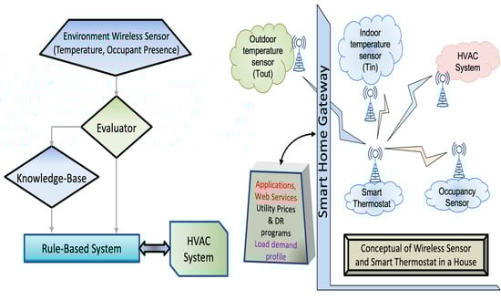
Also known as autonomous control, based on static command control strategies RBCs are not capable of making any adaptive decisions, and, in most uses, algorithms are based on fuzzy logic. Their implementation is simple and flexible compared to other control strategies ^[1][45]. To improve decision-making in an adaptive way and in a stable state, a metaheuristic or homeostatic algorithm is implemented ^[2][3][46,47]. Figure 14 shows an example of the programmable temperature control systems (PTC) in North America, where their automatic adjustment is based on rules associated with high demand, intervening in the adjustments of these meters based on times when users do not make changes ^[4][48].

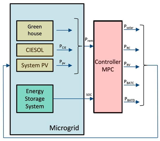
The objective of this type of control is to solve an optimization problem and implement its result. Optimization problems are generally solved in the context of a complex systems control scheme, such as model-based predictive control (MPC) ^[5][49]. The principle of control is to optimize (minimize or maximize) one or more target variables, varying their decision values while satisfying a set of constraints. In the case of the Smart Grid in Figure 25, the conventional approach is to minimize the cost of the operation, which includes different components (fuel, storage, maintenance, policies, cycles, demand, and supply, among others) ^[6][50]. An application of this control has been developed at the Tamil Nadu Institute of Technology and Sciences, India, where a predictive control model called the trust was implemented in the wireless sensor nodes to observe them as energy supply and demand nodes and thus obtain more adequate metrics. The proposed trust model validates compensation failures and data loss failures in smart meters ^[7][51].

Agent-based modeling control systems are intelligent systems consisting of a collection of agents that interact with each other in such a way that the entire system learns and evolves. The term “agent” refers to a computer system capable of performing autonomous actions, which can be divided into different agents, including: controller, central coordination, load, network entry and exit, planner, management, market, regulation, and others ^[8][9][52,53]. These agents communicate with each other to perform coordinated actions, perform complex calculations, and make decisions. These models are more focused on energy management.

They can be used in situations where a fully formulated optimization problem would be impractically complex or where a model of the complete system cannot be known. They are tolerant of errors due to their decentralized control scheme ^[10][11][54,55].

Research carried out at Beihang University in Beijing, China, presents agent-based control as a solution to failures when they are associated with the dynamic load balancing of the smart grid. The agent-based algorithm optimizes groups of nodes called herds based on load compensation using communication architectures ^[12][56]. A similar system for distribution network restoration in future smart grids can be seen in ^[13][57], where the self-repair capacity of future networks will be a must.

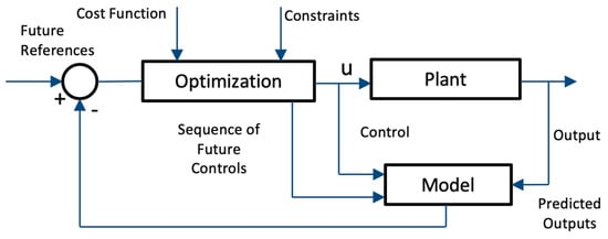
Model-based predictive control is a control strategy based entirely on the dynamic model of the system. In general, it is a linear model that takes as input the current state of the system and external disturbances and generates a future state ^[14][58]. The resulting state is optimized in a prediction horizon of N + 1, and the now-current state (N + 1) with the current and predicted disturbances is introduced into the model, as in Figure 36. The MPC has the advantage of having an account of the future state of the system and future disturbances when making control decisions for the current next step; thus, one can anticipate future events and act on that prior knowledge in the present. An advantage of the predictive control of the model is that it is only as good as the model that is placed in it ^[15][16][59,60].

This type of model is being applied in commercial buildings in Hong Kong for the management of the demand for air conditioners and its relationship with the supply of energy through the Smart Grid. The main objective is to maximize the power reduction based on a predictive profile of the electrical networks as well as maintain the air temperature inside the building. The MPC controller determines the demand control outputs based on the building’s thermal response model ^[17][61].

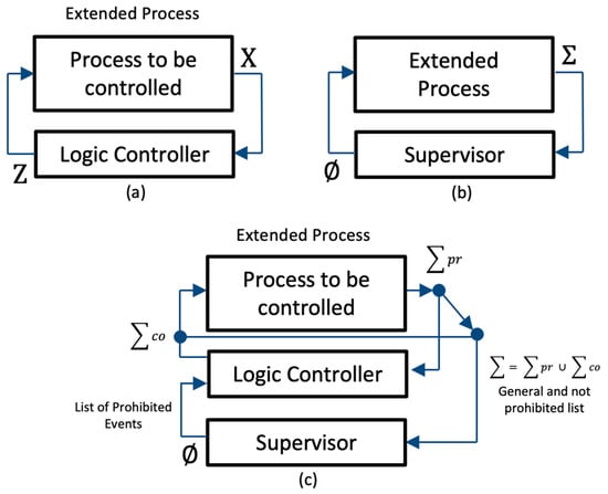
This type of control is based on asynchronous dynamic systems, which evolve according to the occurrence of events ^[19][63]. Its behavior can be described as sequences of events forming a language and thus establishing a process that can be coupled to a supervisor, and this can force the processes to be recurrent. It is present where the Petri nets are perfectly coupled by the supervised control manager, as seen in Figure 47. This type of control was applied in Detroit in the United States by the Department of Electrical and Computer Engineering at Wayne University. Its objective was to avoid overload tripping of circuit breakers through the distribution or output of the overload in the network with the maximum possible power transfer ^[20][64].

Supervised systems are managed via Petri nets since they establish programmable logic rules and define events restricted by actions. These Petri nets have penetrated control systems for failure analysis, financial systems, energy, storage systems, automation systems, and telecommunications through their different forms, such as timed, hybrid, and stochastic Petri nets, combined with other control methods or colored ^[22][23][66,67].

These models can be combined by different techniques, which can be from the same PN family but from different sources, such as Bayesian Petri nets and stochastic Petri nets. In this case, one of them can act as the supervisory PN, which controls the events, and the other PN can generate the model through an algorithm for process control. In addition, a combination of hybrid models can be presented. These can be PNs with a discrete or continuous control model. An applied example of the combination of PN techniques is the modeling of urban traffic systems in the city of Turin, Italy, which uses real-time control strategies. The hybrid model uses timed colored Petri nets (TCPNs; Figure 47, section (b) of reference ^[24][68]) as a system control of entrances and exits in the intersections; these TCPNs establish the possible stopping times, numbers of vehicles, and flow directions, while the vehicular flow on the road has been modeled through a stochastic discrete-time model (Figure 47). Hybrid model validation has shown that relevant traffic dynamics have been considered, but the real-time computational cost is of low latency and time-saving, making it suitable for real-case applications. The above, due to the simulation, can be performed in parallel for the hybrid model ^[24][68].