Your browser does not fully support modern features. Please upgrade for a smoother experience.
Please note this is a comparison between Version 1 by Osama Mohamed ElSahly and Version 2 by Conner Chen.
Traffic incidents have negative impacts on traffic flow and the gross domestic product of most countries. In addition, they may result in fatalities and injuries. Thus, efficient incident detection systems have a vital role in restoring normal traffic conditions on the roads and saving lives and properties. Researchers have realized the importance of Automatic Incident Detection (AID) systems and conducted several studies to develop AID systems to quickly detect traffic incidents with an acceptable performance level. AID can be categorized into four categories: comparative, statistical, artificial intelligence-based and video–image processing algorithms.
- traffic incidents
- automatic traffic incident detection
- incident management
1. Comparative (Pattern Recognition) Algorithms
The comparative algorithms have predefined thresholds that represent normal traffic conditions. The collected traffic flow parameters (i.e., speed, occupancy and/or flow) are compared against these thresholds. If there are significant deviations from these thresholds, incident alarms are triggered [1][2][31,38]. This category includes the California algorithm [3][16], which is the first and the most known algorithm in this category, the Pattern Recognition (PATREG) algorithm [4][39], the All Purpose Incident Detection (APID) algorithm [5][40] and many other algorithms.
The California algorithm, also known as the Traffic Services Corporation (TSC) algorithm, is one of the pioneering algorithms and one of the most known comparative algorithms. It is based on the concept that the occurrence of traffic incidents significantly increases the occupancy in the upstream section of the road while decreasing the occupancy in the downstream section of the road. Thus, it uses the occupancy measured from two adjacent fixed detectors. Three tests are applied to the measured occupancies by the two detectors and if the values from the three tests surpass predefined thresholds, an alarm of incidents is set off [2][6][38,41].
Here, O1 is the difference between the occupancy of the upstream detector and the occupancy of the downstream detector; O2 is the relative difference between the occupancy of the upstream detector and the occupancy of the downstream detector; O3 is the temporal difference in downstream occupancy; T1, T2 and T3 are the test thresholds [7][42].
One of the major drawbacks and limitations of this algorithm is that it depends on the readings of the fixed detectors. Thus, the performance of this algorithm will be significantly affected by any breakdowns or defects in the detectors. In addition, the predefined thresholds are determined based on historical data of normal traffic and incident conditions, which may vary from one location to another. Additionally, the algorithm requires extensive calculations [8][43]. Moreover, in some situations, the traffic might exhibit incident-like patterns even though there is no incident such as the presence of ramps, grade changes or lane drops between detector stations [9][44]. These situations may cause false alarms and thus impact the performance of the algorithm. The algorithm has a good Detection Rate (DR) and acceptable False Alarm Rate (FAR) AR but these are achieved at a cost of delays in detecting the occurrence of incidents and a high Mean Time to Detect (MTTD)TTD that can reach up to 4 min [9][44]. Payne and Tignor modified the original algorithm to overcome some of its limitations and improve its performance. Based on that, 10 algorithms were developed out of it such as California algorithm #7 and California algorithm #8, which were proved to have the best performance [3][10][16,45]. Guo et al. modified the original California algorithm to be able to detect traffic incidents in urban areas instead of freeways [11][46]. Since traffic flow in urban roads is discontinuous and varies with time unlike freeways, which have stable and continuous traffic flow, they suggested using dynamic thresholds, derived from iterative formulas, instead of constant predefined thresholds.
APID algorithm was developed as a component of the COMPASS software, which was designed to be implemented in the traffic management center in Toronto, Canada [5][40]. This algorithm integrates the elements of the California algorithm and expands it to consider different traffic conditions since it has incident detection algorithms for heavy, medium and low traffic conditions plus an incident termination detection routine, a routine to search for the presence of compression waves and persistence of incident condition testing routine [1][6][31,41].
Moreover, the McMaster algorithm was developed to overcome some of the limitations of the California algorithm [12][13][47,48]. Instead of using occupancy only as the input parameter, this algorithm considers the flow, occupancy, and speed from a single station as input parameters. The detection algorithm analyzes the changes in three parameters simultaneously. If a sudden and sharp change in one of the three variables is observed, while the change in the remaining variables is smooth and continuous, this can indicate the occurrence of an incident [13][48]. The algorithm utilizes historical data of normal and incident conditions to develop flow–occupancy–speed charts and sets boundaries between the normal and incident conditions. If the observed traffic parameters exceed the normal condition threshold for consecutive periods, an alarm is triggered to indicate the occurrence of an incident. Using the three parameters together instead of using the occupancy only leads to the main advantage of this algorithm, which is a high incident detection rate compared to the California algorithm. Therefore, this algorithm has higher DR and lower MTTD, compared to the California algorithm. In addition, this algorithm depends on the data obtained from a single station instead of two adjacent stations. Hence, the number of false alarms triggered by the normal variations that mimic incident-like patterns is reduced. However, the major flaw of this algorithm is that the weather conditions can impact its detection capability. The algorithm was assessed during a snowstorm and the FAR was increased significantly because during snowstorms, vehicles had to decrease their speeds sharply and drive more cautiously. This reduction was incorrectly detected as incidents thus the number of FAR was increased in this situation [12][13][47,48].
To alleviate the issue of the random fluctuations that may cause false alarms in the California algorithm, in 1993, Stephanedes and Chassiakos developed the Minnesota algorithm [14][49]. The algorithm collects the occupancy from two adjacent detector stations upstream and downstream over 30 s intervals. The algorithm calculates the average of the spatial occupancy difference between the two stations over six intervals (three minutes). This process is called short-term time averaging. Then, the algorithm inspects the discontinuity in the spatial occupancy difference over the past three minutes. If the spatial difference exceeds certain thresholds, this will trigger an incident alarm. The advantage of using short-term time averaging is to smooth up the random fluctuations in the data, filter the data, and remove the noise that triggers false alarms that affect the detection capability of the algorithm [15][37]. The performance of this algorithm was compared to the performance of the California, Standard Deviation, and Double Exponential algorithms (these will be discussed in the following subsection). This comparison showed that the Minnesota algorithm achieved the highest DR and produced the lowest FAR compared to the other three algorithms [14][49]. However, the main weakness of this algorithm is the detection time, which can be three minutes or more since it collects and evaluates the average spatial occupancy difference over three minutes. In addition, this algorithm depends only on occupancy as the input variable to detect the occurrence of an incident. This may cause undesirable incident alarms especially during low traffic flow. If the flow of the vehicles over the detector stations is low thus the occupancy will be low as well, which may be misclassified as an incident.
The Technical University of Munich developed an Automatic Incident Detection (AID) D system using Bluetooth detectors instead of an inductive loop as part of a project called iRoute [16][50]. These detectors were used to measure the actual travel time of the vehicles and then the speed of the vehicles between two consecutive detector stations, with known distances, can be calculated. A considerable increase in travel time and decrease in speed can be used as a sign of the existence of an incident on the road. The advantage of this system is that it uses Bluetooth detectors instead of inductive loop detectors, which are less expensive, have low installation and maintenance costs, and also have high scanning and detection range compared to inductive loops. Thus, a low number of detectors can provide a wider coverage area. Additionally, their power consumption is very low and the collected data can be easily transferred via The Global System for Mobile Communications (GSM), which has low service costs. Nevertheless, the performance of this system is highly affected by the distance between the Bluetooth detectors since the DR decreases with the increase in the distance between the detectors as the incidents can be smoothed quickly before their impacts reach the downstream detectors [17][51].
2. Statistical Algorithms
These algorithms use statistical techniques to estimate traffic characteristics and compare them with the observed traffic data obtained from the road to determine if there is a statistical difference between them, which indicates potential incidents [1][6][31,41]. The contributions and the limitations of these algorithms are discussed in this subsection. In 1974, the Texas Transportation Institute (TTI) developed the Standard Normal Deviate (SND) Algorithm and applied it on the Houston Gulf Freeway (I-45) [18][14]. This algorithm uses historical data on the traffic parameters and calculates the mean (x0) and the standard deviation (σ) of these variables and then compares them to the current values of the variables collected from the field to calculate the SND using Equation (4).3. Artificial Intelligence Algorithms
With the development of computational intelligence, Artificial Intelligence (AI) and Machine Learning (ML) and ML are used extensively in the transportation sector [25][26][27][77,78,79]. They are used in managing and controlling traffic volume [28][80], predicting the traffic flow of autonomous vehicles [29][81], traffic management and planning [30][31][82,83] and detecting traffic incidents [32][33][34][35][35,84,85,86]. Artificial Intelligence algorithms apply AI and ML models to identify the normal and abnormal traffic patterns and then classify the given input data as either incident or normal conditions [36][87]. These algorithms include Artificial Neural Networks (ANNs), fuzzy logic, random forest, decision trees, support vector machine (SVM) and a combination of these models [1][6][31,41].4. Video–Image Processing Algorithms
CCTV cameras are used for traffic management on roadways. The video–image processing algorithms use traffic videos captured from CCTV cameras installed on the roads to detect traffic incidents [1][37][38][31,72,130]. They break the recorded videos into a sequence of image frames and then extract the background roads and subtract moving vehicles from them. These frames are analyzed by video–image processing algorithms that track the moving vehicles to determine the spatial-temporal characteristics of the traffic variables and then analyze these to identify incident or incident-free states [39][40][131,132]. Figure 14 shows the steps of video–image processing incident detection algorithms.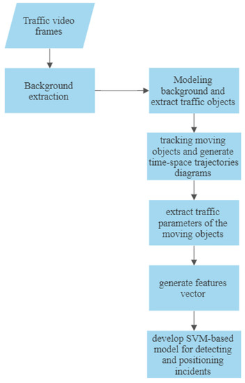
Table 1.
Advantages and disadvantages of incident detection algorithms.
| Category | Contributions and Advantages | Limitations and Drawbacks | |
|---|---|---|---|
| Comparative algorithms | California algorithms | Look for discrepancies in traffic parameters between adjacent loop detectors to identify the presence of an incident [2][3][6][7][8][9][10][11][16,38,41,42,43,44,45,46]. It has good DR and a tolerable FAR. |
It has a long MTTD that can reach about 4 min [9][44]. The performance of the algorithm is affected by any malfunction in any detector. Some factors can cause incident-like patterns and increase the number of false alarms. |
| McMaster algorithms | Overcome the weaknesses of the California algorithm series [12][13][47,48]. It uses the data from a single detector station instead of two adjacent stations and considers the relationship between speed, flow and occupancy. |
It is sensitive to severe weather conditions such as rain or snow, which may result in an increase in the number of false alarms. | |
| Minnesota algorithm | Investigates the discontinuity in the average spatial occupancy difference between the two stations over six intervals. The algorithm uses short-term time averages to smooth up the random fluctuations in the data, filter the data, and remove the noise that triggers false alarms, which affects the detection capability of the algorithm [14][15][37,49]. | The detection time can be three minutes or more. It depends on the occupancy only to detect incidents, which can cause false alarms during low traffic conditions. |
|
| Bluetooth based algorithms | Uses Bluetooth detectors instead of an inductive loop, which provides a reliable, cost-efficient and fast method for detecting traffic incidents or congestion [16][17][50,51]. | Some factors such as detectors spacing, operating conditions, duration and severity of the incident and the location of the incident relative to the detectors can impact the performance of the algorithm. | |
| GPS-based algorithms | Utilizes driver’s mobile phones or GPS trackers in the vehicles to establish spatio-temporal traces of the vehicles to detect traffic congestion and incidents [44][45][52,53]. | The range and the placement of the sensors can affect the efficiency of the sensors or may cause false alarms. | |
| FCD-based algorithms | Uses probe vehicles to collect real-time traffic data and detect the occurrence of incidents. Cost-effective method that can be used instead of fixed detectors [46][47][48][49][50][51][54,55,56,57,58,59]. |
Penetration rate of the tracked vehicles on the road and data latency affect the performance of the algorithm. | |
| V2V- and V2I-based algorithms | Use V2V and V2I communications to monitor traffic and detect incidents and congestion [52][53][54][55][56][57][60,61,62,63,64,65]. | Impacted by the availability of the communications protocols among different entities (vehicles and infrastructure). | |
| Statistical Algorithms | SND algorithm | Evaluates the deviation of a variable from the means to identify potential incidents [1][4][6][18][19][14,31,39,41,66]. | Sensitive to the presence of outliers, which can cause the masking phenomenon. |
| IQD-based algorithm | Overcomes the masking phenomenon in the SND algorithm by using the median or the second quartile instead of the mean and Inter-Quartile score Q instead of the standard deviation to calculate IQD [20][21][22][67,68,69]. | It is prone to swamping phenomenon, which can increase FAR. | |
| DES algorithm | Removes the noise and heterogeneity from the traffic data to clarify the true traffic patterns to help the system to detect incidents easily and reduce false alarms [23][24][58][30,70,71]. | It predicts the traffic variables under normal traffic conditions and assumes that the traffic will follow the predicted pattern over time. Additionally, it requires extensive computational efforts. | |
| Time Series Algorithms | Uses historical data of traffic variables to employ statistical short-term forecasting of normal traffic conditions. Significant deviations between the observed and predicted conditions indicate the existence of incidents [4][6]60][61][,7562][39[23][37][,4159,70],72,73[,74,76]. | Time-consuming and require extensive computational efforts. Additionally, they assume the traffic follows a predictable pattern over time. | |
| Artificial Intelligence Algorithms | ANN algorithms | Uses machine learning to classify the provided traffic data as incident or non-incident situations [1][15][63][64][65][66][,94[,9567][68],9669,97][,9870][,9971][72][19,31,37,93,100,101]. | The accuracy of the algorithm depends on the performance of the model which needs optimization and tuning. There is no rule to determine the structure of the network, the appropriate structure is achieved through trial and error. |
| Fuzzy logic algorithms | Deal with the complex and stochastic nature of traffic variables. They provide the likelihood for an incident [44][73][74][75][76][77][52,114,115,116,117,118]. | The performance depends on the rules and membership functions that are set. They completely depend on human knowledge and expertise. It does not give a clear signal of incident or no incident. |
|
| Support Vector Machine | Provides a computationally efficient nonlinear classifier that can be used in real-time incident detection [32][78][79][80][81][82][83][21,35,119,120,121,122,123]. | The accuracy of the model is highly dependent on the kernel function used. Nevertheless, selecting the appropriate kernel function is complex. SVM is suitable for large datasets because this will make the training process very time-consuming. |
|
| Ensemble Learning Algorithms | Combine multiple machine learning models to build a powerful prediction model that has better predictive performance than any constituent machine learning model alone [19][32][84][85][25,35,66,129]. | The models should be selected carefully to improve the predictive performance of the model. The ensemble can be complex and less interpretable and can cost more time during creating and training. |
|
| Video–image Processing Algorithms | Analyze videos of real-time traffic captured by surveillance cameras to detect traffic congestions and incidents [1][[316][37][38,41,72],130[39][40][41],131,132,133[42][43,134],135]. | The lighting conditions, extreme weather conditions and coverage range of the camera that is used to capture traffic video have a major impact on the algorithm’s performance [6][41]. | |