Your browser does not fully support modern features. Please upgrade for a smoother experience.
Please note this is a comparison between Version 2 by Beatrix Zheng and Version 1 by Junchao Wang.
The quantum computer has been claimed to show more quantum advantage than the classical computer in solving some specific problems. Many companies and research institutes try to develop quantum computers with different physical implementations. Currently, most people only focus on the number of qubits in a quantum computer and consider it as a standard to evaluate the performance of the quantum computer intuitively. However, it is quite misleading in most times, especially for investors or governments. This is because the quantum computer works in a quite different way than classical computers. Thus, quantum benchmarking is of great importance. Currently, many quantum benchmarks are proposed from different aspects.
- quantum computing
- quantum benchmark
- fidelity
- qubit
- quantum circuit
1. Overview of Quantum Benchmarks
In this research, wthe cresearchers classify the benchmarks into three categories: the physical benchmarks, the aggregated benchmarks, and application-level benchmarks. Most news and reports place emphasis on the number of qubits in a quantum processor, which is mostly misleading for those who are not familiar with quantum computing. Definitely, the number of qubits can directly decide the quantum computing power of a quantum computer. Some people intuitively think that the quantum computing power of a quantum computer grows exponentially with the number of qubits. For instance, in 2019, Google first demonstrated “quantum supremacy” with a Sycamore quantum processor having 53 qubits. However, apart from the number of qubits, the noise and the quantum property of the qubits can greatly affect the correctness of the results. Thus, apart from the number of qubits, there are other physical properties that most people are concerned about.
Physical benchmarks include tools, models, and algorithms to reflect the physical properties of a quantum processor. Typical physical indicators of quantum computers include T1, T2, single qubit gate fidelity, two qubit gate fidelity, and readout fidelity. The aggregated benchmarks can help the user to determine the performance of a quantum processor with only one or several parameters. The aggregated metrics can be calculated with randomly generated quantum circuits or estimated based on the basic physical properties of a quantum processor. Typical aggregated benchmarks include quantum volume (QV) and algorithmic qubits (AQ). The application-level benchmarks refer to the metrics obtained by running real-world applications on the quantum computer. Many existing works propose using real world applications to benchmark the quantum computer’s performance because they assume that random circuits cannot reflect a quantum computer’s performance accurately. An overview of the existing quantum benchmarks is shown in Figure 1.
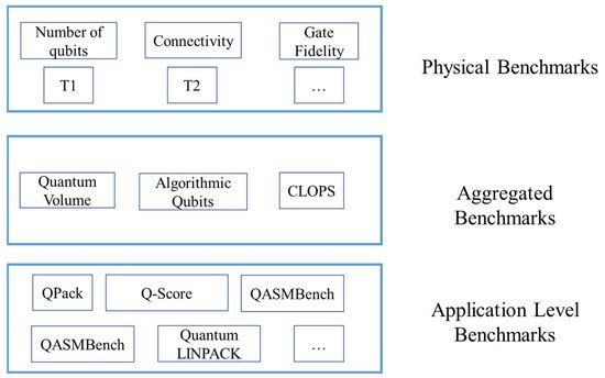
Figure 1.
Overview of the quantum benchmarks.
2. Physical Benchmarks
Different physical implementations are concerned with different aspects of a quantum computing system. For instance, the trapped ion-based quantum computer focuses more on the stability of the trap frequency, the duration of a gate operation, and the stability of the control lasers. The superconducting quantum computers’ performance is affected by the controllability and scalability of the system. Mostly, they are affected by the precision of the Josephson junction, anharmonicity, and gate duration [8][1].
In general, the quantum computation systems are concerned with the quantum correlations and controlling operation precision. In a superconducting quantum computer, generally researchers from the background of quantum information focus more on physical properties of quantum computers, such as the T1, T2, number of qubits, connectivity, single qubit gate fidelity, two qubit gate fidelity, and readout fidelity.
The indicators for quantum computers of IBM’s online quantum cloud (Table 1, from [9][2]) is shown in the following table.
Table 1.
IBM quantum cloud’s performance metrics. Avg stands for average; N/A means not applicable.
| Q-Score | |||||
| TSP and Max-Cut | VQC | Q-Score | |||
| [28] | [14] | F-VQE | Max-Cut | VQC | N/A |
| [29] | [15] | Variational quantum factoring (VQF) and fermionic simulation | Variational quantum factoring (VQF) and fermionic simulation | VQC | The effective fermionic length of the device |
| [30] | [16] | Machine learning application | Approximating an unknown probability distribution from data | Data-driven quantum circuit learning algorithm (DDQCL). | qBAS (bars and stripes) score |
| [31] | [17] | 3 application-motivated quantum circuit | N/A | The quantum circuits include: the deep class of the quantum circuit is taken from the state preparation in the VQE (variational quantum eigensolver) algorithm; the shallow class of quantum circuits refers to the circuits whose depths increases slowly with the growth of width (number of qubits); square is inspired by the quantum volume benchmark. | Heavy output generation probability, cross-entropy difference and l1-norm distance |
| [32] | [18] | Application-oriented performance benchmarks | N/A | The quantum circuits of the benchmark include: shallow simple Oracle-based algorithms, quantum Fourier transform (QFT), Grover’s search algorithm, phase and amplitude estimation, Monte Carlo sampling, variational quantum eigensolver (VQE), and Shor’s order finding. | The quality and execution time |
| [33] | [19] | Quantum LINPACK | Dense random matrix in a quantum problem | RAndom Circuit Block-Encoded Matrix (RACBEM). | N/A |
| [34] | [20] | Quantum chemistry benchmark | Electronic structure calculation instances | reduced unitary coupled cluster ansatz (UCC, a state preparation circuit) and hardware-efficient ansatz (Variational Quantum Eigensolver, VQE). | Performance and accuracy |
| [35] | [21] | QASMBench | N/A | Quantum circuits are taken from chemistry, simulation, linear algebra, searching, optimization, arithmetic, machine learning, fault tolerance, cryptography. | circuit width, depth, gate density, retention lifespan, measurement density and entanglement variance |
| Name | Number of Qubits | QV | Avg.T1 (μs) | Avg.T2 (μs) | Avg.Readout Fidelity | Avg.CNOT Fidelity |
|---|---|---|---|---|---|---|
| brooklyn | 65 | 32 | 77.1686 | 74.6345 | 0.9682 | 0.9746 |
| manhattan | 65 | 32 | 110.1959 | 101.6078 | 0.9761 | 0.9543 |
| hanoi | 27 | 64 | 123.3959 | 93.4341 | 0.9837 | 0.991 |
| sydney | 27 | 32 | 266.1433 | 256.6081 | 0.9833 | 0.9898 |
| peekskill | 27 | N/A | 97.4474 | 107.0911 | 0.9821 | 0.9896 |
| cairo | 27 | 64 | 76.01 | 97.6543 | 0.9796 | 0.989 |
| toronto | 27 | 32 | 180.3614 | 155.1329 | 0.9869 | 0.9814 |
| kolkata | 27 | 128 | 70.3363 | 75.2432 | 0.9698 | 0.9536 |
| mumbai | 27 | 128 | 117.2574 | 92.1067 | 0.9484 | 0.9526 |
| montreal | 27 | 128 | 81.004 | 104.678 | 0.938 | 0.4972 |
| guadalupe | 16 | 32 | 132.6257 | 40.5357 | 0.977 | 0.9896 |
| lagos | 7 | 32 | 158.6 | 57.702 | 0.9697 | 0.9912 |
| jakarta | 7 | 16 | 74.214 | 104.008 | 0.9728 | 0.9895 |
| perth | 7 | 32 | 155.0078 | 92.217 | 0.9118 | 0.9894 |
| casablanca | 7 | 32 | 82.2681 | 96.0744 | 0.9696 | 0.9883 |
| nairobi | 7 | 32 | 86.5337 | 107.1733 | 0.9428 | 0.9878 |
| quito | 5 | 16 | 130.2629 | 100.9629 | 0.9859 | 0.9932 |
| santiago | 5 | 32 | 105.2286 | 98.9143 | 0.9633 | 0.9909 |
| manila | 5 | 32 | 100.56 | 101.29 | 0.9739 | 0.99 |
| lima | 5 | 8 | 84.0278 | 84.4122 | 0.9829 | 0.9891 |
| belem | 5 | 16 | 75.936 | 94.722 | 0.9676 | 0.9828 |
| bogota | 5 | 32 | 92.454 | 124.096 | 0.959 | 0.9794 |
| armonk | 1 | 1 | 118.1 | 149.22 | 0.967 | N/A |
3. Aggregated Benchmarks
Each metric can reflect one aspect of the one or two qubit’s performance. However, the quantum processor consists of many qubits connected with different topology. To better evaluate the performance of a quantum computer, people try to propose an aggregated metric to directly reflect the performance of a quantum processor.
3.1. Quantum Volume
When building a larger-scale quantum computer, its performance is susceptible to many factors, such as the number of qubits, connectivity of qubits, and error rate when applying quantum gates. To this end, IBM proposed the quantum volume (QV) [17][3], a metric used to represent the performance of a quantum computer. Quantum volume is calculated as 2k, where k is the largest number of a quantum circuit consisting of k qubits and k-layer gate operations taken from the Haar-random SU(4) unitaries. The QV considers both the number of qubits and the quality of gate operations and measurement. After running the k-layer quantum circuits, the “correct” measured results (heavy output) should be above a certain threshold [18][4]. Thus, it means that the higher gate fidelity can lead to larger QV.
After the first proposal of quantum volume, many researchers address the flaws of QV. For instance, the quantum circuit used by the quantum volume is a “square”, since it constrains the minimum circuit depth and number of qubits. For some algorithms, the quantum circuit is not “square”. In the factorization algorithm (Shor algorithm), the width of the quantum circuit is n, but the depth is n3 [19][5]. So, QV may not necessarily be the widely accepted quantum benchmarking indicator. Moreover, the QV can be very large in some cases. For instance, the scale of QV reaches almost 4 million for an ion-trap quantum computer [20][6]. However, for superconducting computers, the QV generally only reaches 128 maximally. This is mainly because the gate fidelity of superconducting quantum computers is below the gate fidelity of the trapped-ion quantum computers. Additionally, the QV is calculated as 2 to the power of the number of high-quality qubits. Thus, the QV can be quite large in trapped-ion quantum computers. Although QV has drawbacks, it is a great endeavor to draw people’s attention to the problems in a quantum computer, instead of only focusing on the number of qubits in a quantum computer [21][7].
3.2. Algorithmic Qubits
The QV metric will become very large because it is exponential to the number of effective width and length for a given circuit. Since the IonQ’s quantum computer has comparatively high gate fidelity, the QV numbers will grow quickly. To address the shortcomings of quantum volume, IonQ introduces a new benchmark—algorithmic qubits. The number of algorithmic qubits (AQ) determines how big a quantum circuit can be executed on a quantum computer. AQ considers error correction and is directly related to the number of qubits. The IonQ’s roadmap for their future quantum computers is based on the AQ metric [22][8]. IonQ also publishes an online tool for allowing users to calculate the AQ value of a quantum computer, given its basic properties [23][9].
3.3. Mirroring Benchmarks
Proctor et al. concluded that the standard error metrics obtained through random disordered program behavior cannot accurately reflect the performance for some real-world problem [24][10]. To provide direct insight into a processor’s capability, Proctor et al. built the benchmarks starting from the quantum circuits of varied sizes and structures and transformed the circuits to the mirror circuits that can be efficiently verifiable. In ref. [24][10], the quantum benchmarks include: the volumetric circuit benchmarks (referring to the IBM quantum volume [19][5]), the randomized mirror circuits (alternating the layers of randomized Pauli gates and Clifford gates chosen from a sampling distribution), and the periodic mirror circuits (consisting of iteratively germ circuits that can amplify the errors). Proctor et al. assumed that the mirror benchmarks are more efficient, reliable, and scalable for predicting the performance of quantum computing in solving real world problems. The randomized mirror circuit benchmarks are evaluated on twelve processors of IBM quantum computers and Rigetti quantum computers. Their experimental results show that current quantum computing hardware suffers from complex errors. The errors in the structured quantum circuits of real-world applications are quite different from the standard error metrics from random benchmarking techniques. The capability of a quantum processor can be reflected by a similar approach, such as quantum volume. The results also imply that whether a quantum circuit can be successfully run on a quantum processor depends on the circuit’s shape and the exact arrangement of the quantum gates.
3.4. CLOPS
In [25][11], Wack et al. identified three key attributes for evaluating the performance of a quantum computer: quality, speed, and scale. The quality is measured by the quantum volume deciding the maximum size of quantum circuit that can be executed. The scale can be represented by the number of qubits. The speed is measured by the circuit layer operations per second (CLOPS). The CLOPS metric considers the interaction between classical computing and quantum computing because real-world applications include both the classical processing and the quantum processing. The CLOPS is defined as the number of QV layers executed per second. The CLOPS benchmark includes 100 parameterized templated circuits. It allows the system taking all optimizations during the data transfer of circuits and results, run-time compilation, latencies in loading control electronics, initialization of control electronics, gate times, measurement times, reset time of qubits, delays between circuits, parameter updates, and results processing.
Limitations of the benchmark: The CLOPS mostly focuses on the quantum computing part. The computation accounts only for the runtime compilation and optimization. Thus, in CLOPS, the classical computation serves as assistance to the quantum computing. Improvement in the performance of the classical part can barely contribute to the improvement of CLOPS. For an extreme case, when all applications are executed in a classical computer, the CLOPS will be zeroed, since no quantum circuits are executed. Moreover, the CLOPS only considers the time for executing an application, but the quality of qubits and gate operations is reflected in other parameters. From the experimental results of [25][11], the weresearchers can see that the quantum circuit execution time only takes quite a small proportion (less than 1%) of the total execution time.
4. Application-Based Benchmarks
The physical properties of a quantum computer can affect its performance. However, it is difficult to determine whether a quantum computer outperforms another only based on these properties. For instance, a quantum computer “A” has less qubits, but the qubits’ quality of another quantum computer “B” is higher. If a quantum application needs more qubits, then “A” is preferred. If a quantum application requires the qubits’ quality to be higher, then “B” is preferred. Therefore, some researchers propose to evaluate the performance of a quantum computer with a real-world quantum application.
A summary of the application-based quantum benchmarks is shown in Table 2. In Table 2, wthe cresearchers can see that most quantum benchmarks consider the typical combinational optimization problems and use variational quantum circuits (VQC) to solve the problem. This is mainly because the combinational optimization problems can be widely used in many real-world scenarios, such as traffic engineering and flight scheduling. Moreover, the variational quantum solutions, such as quantum approximation optimization algorithm (QAOA) and variational quantum eigensolver (VQE) are popular, due to the possibility to obtain a useful result on NISQ devices. Thus, most people believe that, in the NISQ era, the variational quantum solution will remain the most effective solution.
Table 2.
Summary of the application-based quantum benchmarks.
References
- How Is the Quantum Computer Performance Assessed. Available online: https://quantum.ieee.org/education/quantum-supremacy-and-quantum-computer-performance (accessed on 9 July 2021).
- IBM Quantum Experience. Available online: https://quantum-computing.ibm.com (accessed on 17 November 2021).
- Bishop, L.S.; Bravyi, S.; Cross, A.; Gambetta, J.M.; Smolin, J. Quantum Volume. 2017. Available online: https://storageconsortium.de/content/sites/default/files/quantum-volumehp08co1vbo0cc8fr.pdf (accessed on 17 November 2021).
- Cross, A.W.; Bishop, L.S.; Sheldon, S.; Nation, P.D.; Gambetta, J.M. Validating quantum computers using randomized model circuits. Phys. Rev. A 2019, 100, 032328.
- Blume-Kohout, R.; Young, K.C. A volumetric framework for quantum computer benchmarks. Quantum 2020, 4, 362.
- IonQ Quantum Computer 4 Million Quantum Volume. Available online: https://www.nextbigfuture.com/2021/03/ionq-quantum-computer-4-million-quantum-volume-and-16x-error-correction.html (accessed on 28 March 2021).
- Scott Aaronson: Turn Down the Quantum Volume. Available online: https://www.scottaaronson.com/blog/?p=4649 (accessed on 1 March 2020).
- Scaling IonQ’s Quantum Computers: The Roadmap. Available online: https://ionq.com/posts/december-09-2020-scaling-quantum-computer-roadmap (accessed on 1 December 2020).
- Algorithmic Qubit Calculator. Available online: https://ionq.com/algorithmic-qubit-calculator/ (accessed on 1 March 2021).
- Proctor, T.; Rudinger, K.; Young, K.; Nielsen, E.; Blume-Kohout, R. Measuring the Capabilities of Quantum Computers. Nat. Phys. 2020, 18, 75–79.
- Wack, A.; Paik, H.; Javadi-Abhari, A.; Jurcevic, P.; Faro, I.; Gambetta, J.M.; Johnson, B.R. Quality, Speed, and Scale: Three key attributes to measure the performance of near-term quantum computers. arXiv 2021, arXiv:2110.14108.
- Mesman, K.; Al-Ars, Z.; Mller, M. QPack: Quantum Approximate Optimization Algorithms as universal benchmark for quantum computers. arXiv 2021, arXiv:2103.17193.
- qScore. Available online: https://github.com/myQLM/qscore (accessed on 1 June 2021).
- New Cambridge Quantum Algorithm Sets a Benchmark in Performance and Effectively Outperforms Existing Methods. Available online: https://quantumzeitgeist.com/new-cambridge-quantum-algorithm-sets-a-benchmark-in-performance-and-effectively-outperforms-existing-methods/ (accessed on 1 June 2021).
- Dallaire-Demers, P.L.; Stęchły, M.; Gonthier, J.F.; Bashige, N.T.; Romero, J.; Cao, Y. An application benchmark for fermionic quantum simulations. Am. Phys. Soc. 2021, arXiv:2003.01862.
- Benedetti, M.; Garcia-Pintos, D.; Perdomo, O.; Leyton-Ortega, V.; Nam, Y.; Perdomo-Ortiz, A. A generative modeling approach for benchmarking and training shallow quantum circuits. NPJ Quantum Inf. 2019, 5, 45.
- Mills, D.; Sivarajah, S.; Scholten, T.L.; Duncan, R. Application-Motivated, Holistic Benchmarking of a Full Quantum Computing Stack. Quantum 2020, 5, 415.
- Lubinski, T.; Johri, S.; Varosy, P.; Coleman, J.; Zhao, L.; Necaise, J.; Baldwin, C.H.; Mayer, K.; Proctor, T. Application-Oriented Performance Benchmarks for Quantum Computing. arXiv 2021, arXiv:2110.03137.
- Dong, Y.; Lin, L. Random circuit block-encoded matrix and a proposal of quantum LINPACK benchmark. Phys. Rev. A 2020, 33, 062412.
- McCaskey, A.J.; Parks, Z.P.; Jakowski, J.; Moore, S.V.; Morris, T.; Humble, T.S.; Pooser, R. Quantum chemistry as a benchmark for near-term quantum computers. npj Quantum Inf. 2019, 5, 99.
- Li, A.; Krishnamoorthy, S. QASMBench: A Low-level QASM Benchmark Suite for NISQ Evaluation and Simulation. arXiv 2020, arXiv:2005.13018.
More