Novel Pooling Methods for Convolutional Neural Networks

Novel Pooling Methods for Convolutional Neural Networks: Comparison

Please note this is a comparison between Version 2 by Amina Yu and Version 1 by Ali Arshad.

Neural network computational methods have evolved over the past half-century. In 1943, McCulloch and Pitts designed the first model, recognized as the linear threshold gate. Hebbian developed the Hebbian learning rule approach for training the neural network. However, would the Hebbian rule remain productive when all the input patterns became orthogonal? The existence of orthogonality in input vectors is a crucial component for this rule to execute effectively. To meet this requirement, a much more productive learning rule, known as the Delta rule, was established. Whereas the delta rule poses issues with the learning principles outlined above, backpropagation has developed as a more complicated learning approach. Backpropagation could learn an infinite layered structure and estimate any commutative function. A feed-forward neural network is most often trained using backpropagation (FFNN).

pooling methods
convolutional neural network
overfitting

1. Novel Pooling Methods

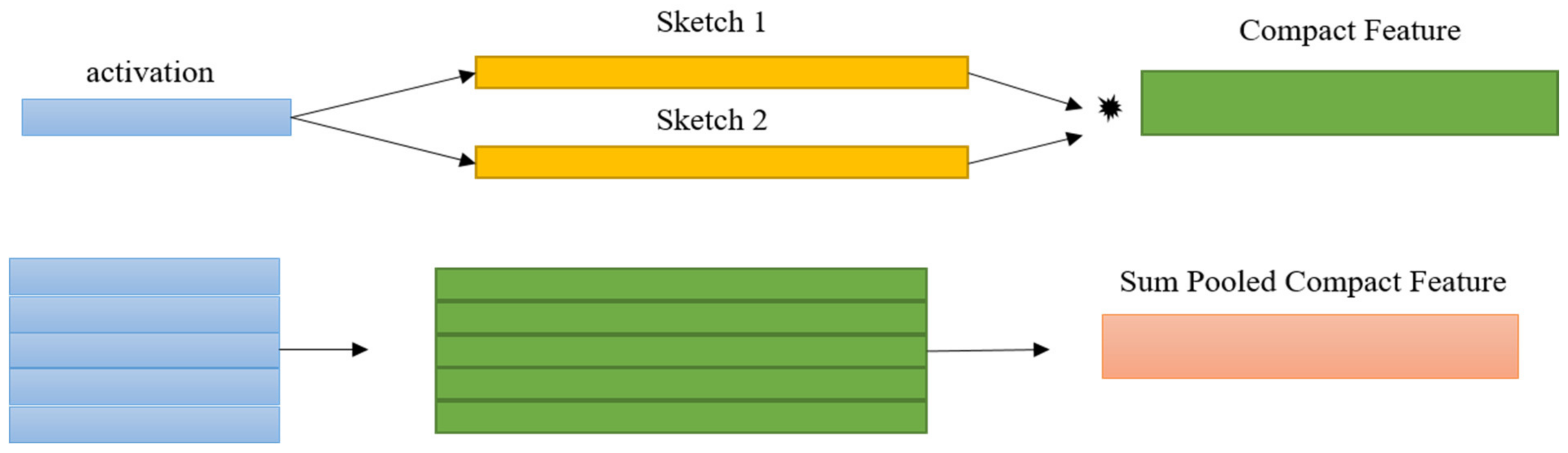
1.1 Compact Bilinear Pooling

Bilinear methods have been shown to perform well on several visual tasks, including semantic segmentation, fine-grained classification, and facial detection. End-to-end backpropagation is being used to train the compact bilinear pooling technique that allows for a low-dimensional and highly discriminatory image representation. This approach of pooling is also employed in [52,53]^[1][2].

For the last convolutional feature, this strategy is suggested to achieve global heterogeneity and rich representations, which attained cutting-edge performance in several multidimensional datasets. However, since computing pairing interaction between channels produces great complexity, dimension reduction methods have been presented. Low-rank bilinear pooling (Figure 51) shows a schematic representation of compacted bilinear pooling. End-to-end backpropagation has been used to train this pooling technique, which allows for a low-dimensional yet highly discriminatory image representation.

Figure 51.

Image identification using the compact bilinear pooling method.

1.2. Spectral Pooling

Ripple et al. [54]^[3] proposed a novel pooling approach that included the concept of dimension reduction by shrinking the frequency domain representation of the data. Let h*w be the appropriate output feature map parameters and let x Rm*m be the given input map. The given input map is first treated with a discrete Fourier transform (DFT) after during which a frequencies representation submatrix of h*w size is eliminated from the center. Finally, inverse DFT is used to convert the h*w submatrix back into image pixels. By implementing a threshold-based filtering methodology, spectral pooling retains more information over max pooling for the very same output dimension. It fixes the problem of the output map’s dimensions being reduced significantly.

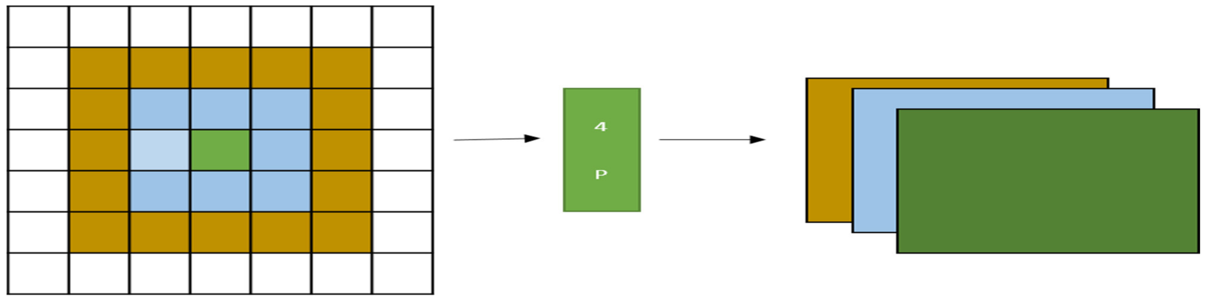
1.3. Per Pixel Pyramid Pooling

To obtain the requisite receptive field size, a wider pooling window could have been used as contrasted to a stride and a narrow pooling window. While using a large single pooling window, finer details may be lost. As a consequence, successive pooling with various window dimensions is conducted, and the results are concatenated to construct additional feature maps. The material from broad to fine scales is presented in the feature maps that emerge. The multi-scale pooling process can be carried out by each pixel without strides. The preceding is the formal definition of per-pixel pyramid pooling [55]^[4].

P^4p (F, S) = [P (F, S1)… P (F, S_m)]

P (F, Si) is a pooling process with a size of Si and a stride of 1, and s is a vector with an element count of M. To be clear, one channel of the extracted features is shown in Figure 6 2 to demonstrate the pooling process; the other channels obtained similar findings.

Figure 62.

Representation of the 4P module with the pooling size vector s = [5, 3, 1].

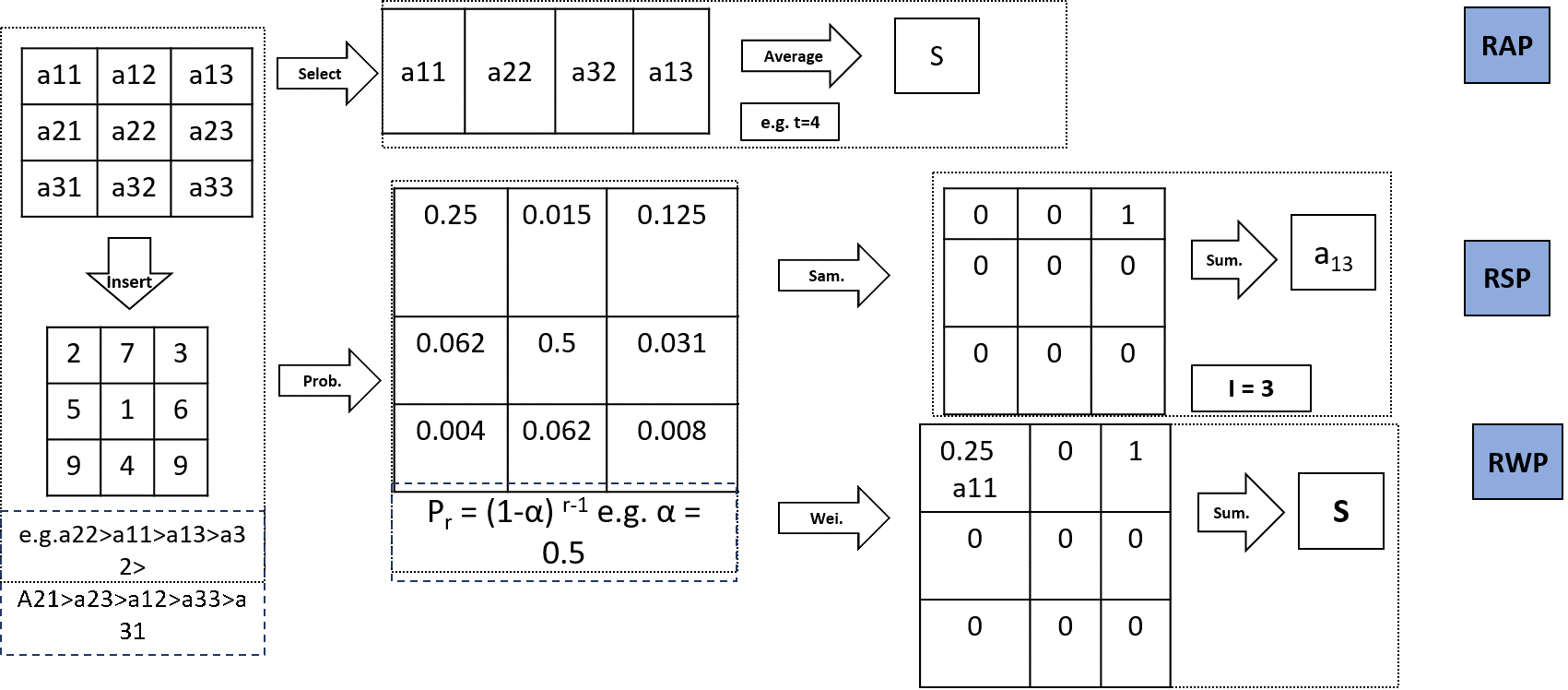
1.4. Rank-Based Average Pooling

The proposed pooling evaluates the average performance for practically zero negativity activation functions, which could also cause the loss of racist and discriminatory data by downplaying higher activation levels. Likewise, in max pooling, non-maximum activations are eliminated, leading to data loss. A rank-based average pooling layer can overcome the challenges of information loss imposed on both max pooling and average pooling layers (RAP) [56]^[5]. The outcome of the RAP can be stated as Equation (8):

The ranks boundary, which defines the categories of activations used during averaging, is represented by t. In feature maps, R stands for the pooling regions j, and t stands for the index of each activation inside of it. S_j and a_i, within this order, reflect the rank of activation I and the value of activation I. When t = 1, max pooling is established. According to Shi et al. [37]^[6], limiting t to a median value achieves good performance and a good balance between max pooling and average pooling. Therefore, RAP has better discriminative power than traditional pooling methods and is a perfect combination of maximum and average pooling. Figure 7 3 depicts a simulation of rank-based pooling in operation.

Figure 73. Rank-based average pooling: rankings are presented in ascending order, and activations for a pooling area are listed in descending order. The pooling output is calculated by averaging the four largest activations, since t = 4.

1.5. Max-Out Fractional Pooling

The concept of fractional pooling applies to the modification of the max pooling score. IHerein this case, the multiplication factor (α) can only take non-integer values such as 1 and 2. The location of the pooling area and its random composition are, in fact, factors that contribute to the uncertainty provided by the largest max pooling. The region of pooling can be designed randomly or pseudo-randomly, with overlaps or irregularities, employing dropout and trained data augmentation. According to Graham B. et al. [57]^[7], the design of fractional max pooling with an overlapping region of pooling demonstrates greater performance than a discontinuous one. Furthermore, they observed that the results of the pooling region’s pseudo-random number selection with data augmentation were superior to those of random selection.

1.6. S3Pooling

Zhai et al. in 2017 presented the S3Pool method, a novel approach to pooling [58]^[8]. The pooling process is performed under this scheme in two stages. On each one of the preliminary phase feature maps (retrieved from the convolutional layer), the execution of max pooling is performed by stride 1. The outcome of step 1 is down sampled using a probabilistic process, in comparison to step 2, which first partitions the feature map of size X × Y into a preset set of horizontal (h) and vertical (v) panels. V is y/g and H is x/g. The following figure illustrates a schematic of S3Pooling. The working of S3 pooling is referred in Figure 84.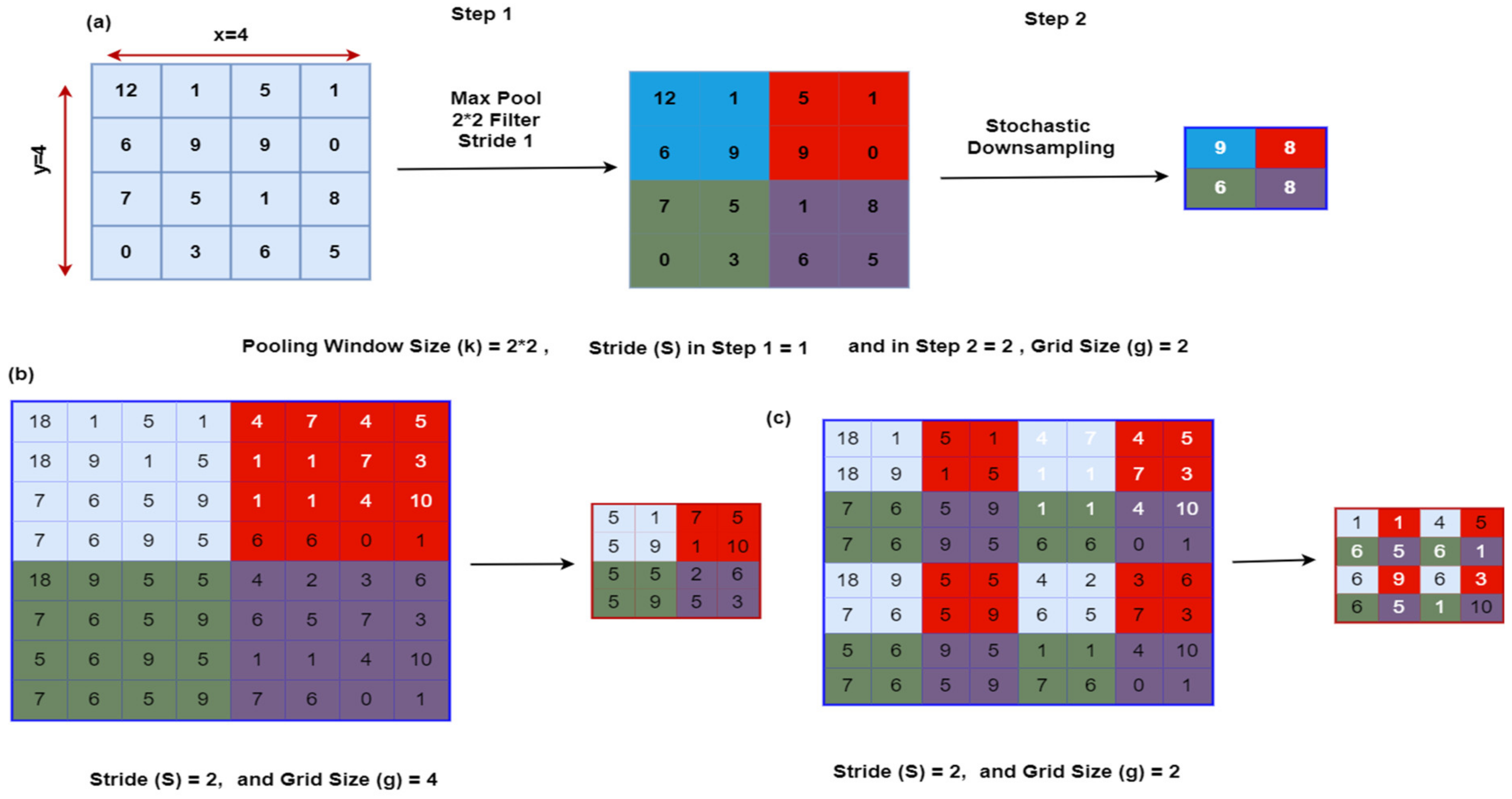

Figure 84. Working of S3 pooling mechanism. The dimension of the feature map in this example is 4 × 4, with both x and y = 4 represented in (a). The max pooling operation in step 1 uses stride 1, and there is no padding at the border. The grid size and stride should both be 2 in step 2. There will be two horizontal (h) and vertical (v) strips. In step 2, a stochastic downsampling is used to represent the rows and columns that were randomly chosen to build the feature map. Flexibility to change the grid size in step 2 in order to control the distortion or stochasticity is represented in (b,c).

Xu et al. [59]^[9] executed tests for the CIFAR-10, CIFAR-100, and SIT datasets using both network in the network (NIN) and residual network architectures to test the effectiveness of S3Pool in comparison to other pooling techniques (ResNet). According to the experimental observations, S3Pool showed better performance than NIN and ResNet with dropout and stochastic pooling, even when flipping and cropping were used as data augmentation techniques during the testing phase.

1.7. Methods to Preserve Critical Information When Pooling

Improper pooling techniques can lead to information loss, especially in the early stages of the network. This loss of information can limit learning and reduce model quality [60,61]^[10][11]. Detail-preserving clustering (DPP) [62]^[12] and local importance-based clustering (LIP) [63]^[13] minimize potential information loss by preserving key features during pooling operations. These approaches can also be known as soft approaches. Large networks require a lot of memory and cannot be started on devices with limited resources. One way to solve this problem is to quickly down sample to reduce the number of layers in the network. Poor performance may be the result of information loss due to the large and rapid reduction of the feature maps. RNNPool [64,65]^[14][15] attempts to solve this problem using a recursive down sampling network. The first recurrent network highlights feature maps and the second recurrent network summarizes its results as pooling output.

2. Advantages and Disadvantages of Pooling Approaches

The upsides and downsides of pooling operations in the numerous CNN-based architectures is discussed in Table 1, which would help researchers to understand and make their choices by keeping in mind the required pros and cons. Max pooling has indeed been applied by several researchers owing to its simplicity of use and effectiveness. Detail analysis was performed for further clarification of the topic.

Table 1.

Advantages and disadvantages of different pooling approach in CNN.

Type of Pooling	Advantages	Drawbacks	References
Max Pooling	-

that the primary aim of this study it is to fairly assess the influence of the pooling strategies in the CNNs, not to establish the optimum classification architecture. Table 2 evaluates the effectiveness of different pooling approaches on standard datasets including MNIST, CIFAR-10, and CIFAR-100. The architecture and the forms of activation functions that have been used to implement these techniques are presented in the following table. In Table 2, it is shown that for the MNIST dataset, average pooling performed the worst, with an error rate of 0.83%. Furthermore, in comparison to other pooling methods, gated pooling was a significant improvement where the average and maximum pools were responsively combined. With a difference of 0.01%, mixed, tree max average pooling, and fractional max pooling were followed in order by the performance of gated pooling. These pooling strategies’ outstanding regularization and generalization capabilities were validated by their effective implementation. In conclusion, the NIN and max out networks’ respectively showed a strong performance and error frequencies of 0.45% and 0.47%. Unfortunately, their performance was still inadequate to what was achieved while pooling methods. It was found that for MNIST datasets, using the same network with ReLU activation, rank-based pooling (RSP) gave a higher error rate than the error rate provided by random pooling in the range of 0.42% to 0.59%.

Table 2.

Comparing performance of various pooling methods on different standard datasets.

Pooling Methods	Architecture	Activation Function	Error Rate of Different Datasets			Accuracy	Reference
Pooling Methods	Architecture	Activation Function	MNIST	CIFAR-10	CIFAR-100	Accuracy	Reference
	Performs more effectively when integrated with simple classifiers and sparse code. - It complements sparse representations due to statistical features. - Eradicating no maximal elements might expedite calculation for upper layers.	- Deterministic in spirit. - The distinguishing characteristics vanish when the majority of the elements in the pooling region are available in significant magnitudes.	[38,^[	Gated Method¹⁶39]^][17]
6 Convolutional Layers	RELU	0.29	7.90	33.22	88% (Rotation Angle)	^[	^32]	Average Pooling	- Easily understandable. - Execution is uncomplicated.	- Forthcoming in spirit. - If minor magnitudes are considered, the contrast is reduced.	[37,38,40,41,56,²42,^][343,44,45,46,47,48,^][449,^][950,^]51,52,^[10][11][12
Mixed Pooling	6 Convolutional Layers	^]	RELU^[¹³^]^[53,¹⁶54,55,^]^[¹⁸^]^[19]^[20]^[21]57,^[58,59,^5][60,^6][[22][2361,^7][25][26]62,^][24[27][2863]^{[1][8]][][29]}
0.30	8.01	33.35	90% (Translation Angle)	Gated Max Average	- Responsive in style. - It is adaptive in whether the volume fraction can fluctuate based on the properties of the pooling region.			- Produces additional training parameters.	[41]^[
Max Pooling	6 Convolutional Layers	¹⁹	RELU^]
0.32	7.68	32.41	93.75% (Scale Multiplier)	Mixed Max Average	- Stochastic pooling. - Facilitates in the problem of overfitting avoidance.	- Once it has been learned, the mix proportion does not really respond and adapt to the attributes of the region being integrated.	[
Max + Tree Pooling	6 Convolutional Layers	42	93.75% (Scale Multiplier)	RELU]^[20]
0.39	9.28	34.75	Pyramid Pooling	- Flexibility to manage input of any size. - Spatial bins with multiple levels. - Responsiveness to the image scales of an input.	- Deep networks’ training step involves complex implementation.	[43]^[21]
Mixed Pooling	6 Convolutional Layers (Without data Augmentation)	RELU	10.41	12.61	37.20	91.5%	[34]^[33]	Stochastic Pooling	- Stochastic procedure. - It is conceivable to use non-maximal activations. - Feasibility of integrating any regularization method, including dropouts, data augmentation, loss tangent, etc. - There seems to be no hyper-parameter to specify. - Lower computational complexity.
Stochastic Pooling		- Complicated to interpret. - Extraneous to words negative activations. - Due to the lack of training data, overfitting occurs because strong activations primarily work in process updating.	3 Convolutional Layers	- Scaling challenge.	[44]	RELU^[22]
0.47	15.26	42.58	---------	[	36	]	^[31]	Tree Pooling	- Flexible to adapt in nature. - Differentiable in perspective among both parameters as well as inputs. - Effective at the network’s lower tiers.	- Inefficient due to thick layers of the network.	[41,66]^[19][30]
Average Pooling	6 Convolutional Layers	RELU	0.83	[	36	]	^[31]	19.38	47.18	---------	Fractional Max Pooling	- Stochastic method. - Choice of the pooling region via pseudo-randomness or randomness. - Appropriate use of data augmentation and pseudo-random selection. - Overlapped rather than disjointed fractional max pooling proved to be more efficient.
Rank-Based Average Pooling (RAP)		-	3 Convolutional Layers	Arbitrarily selecting the pooling zone significantly affects model performance in addition to data augmentation. - The disjointed fractional max pooling leads to significant degradation.	[36]^[31]
RELU	0.56	18.28	46.24	---------	[	37	]^[6]	S3Pool	- Simple to learn and use. - Rapid computations while training. - Extrudes in the extent of distortions. - Implement data augmentation at the levels of the pooling layer to give it strong generalization performance. - Compared to max pooling, considerably increases the computational burden.	- Depending on the design for which it is being employed, the grid size should be adequately specified in each pooling layer. - A greater grid size potentially results in increased testing error.	[37]^[6]
Rank-Based Weighted Pooling (RWP)	3 Convolutional Layers	RELU	0.56	Rank-Based Average Pooling				- For object recognition tasks, it is implemented. - It empowers us to reuse the convolution network’s feature map. - It provides an opportunity to train object detection systems from beginning to end, significantly shortening test and training periods.	- Performance issues can arise while generating lots of regions of interest. - Computing frequency falls short of the expectations. - End-to-end training, or training each aspect of the system in one go, is not practicable but could produce much-enhanced results.	[45]^[23]

Performance Evaluation of Popular Pooling Methods

The performance among the most latest pooling methods has been investigated systematically for the purpose of image classification in this section. WeIt would like tobe emphasized

19.28
48.54
---------
Rank-Based Stochastic Pooling (RSP)
3 Convolutional Layers	RELU	0.59	17.85	45.48	---------
Rank-Based Average Pooling (RAP)	3 Convolutional Layers	RELU (Parametric)	0.56	18.58	45.86	---------
Rank-Based Weighted Pooling (RWP)	3 Convolutional Layers	RELU (Parametric)	0.53	18.96	47.09	---------
Rank-Based Stochastic pooling (RSP)	3 Convolutional Layers	RELU (Parametric)	0.42	14.26	44.97	---------
Rank-Based Average Pooling (RAP)	3 Convolutional Layers	Leaky RELU	0.58	17.97	45.64
Rank-Based Weighted Pooling (RWP)	3 Convolutional Layers	Leaky RELU	0.56	19.86	48.26	---------
Rank-Based Stochastic Pooling (RSP)	3 Convolutional Layers	Leaky RELU	0.47	13.48	43.39	---------
Rank-Based Average Pooling (RAP)	Network in Network (NIN)	Leaky RELU	---------	9.48	32.18	---------	[37]^[6]
Rank-Based Weighted Pooling (RWP)	Network in Network (NIN)	Leaky RELU	---------	9.34	32.47	---------
Rank-Based Stochastic Pooling (RSP)	Network in Network (NIN)	Leaky RELU	---------	9.84	32.16	---------
Rank-Based Average Pooling (RAP)	Network in Network (NIN)	RELU	---------	9.84	34.85	---------
Rank-Based Weighted Pooling (RWP)	Network in Network (NIN)	RELU	---------	10.62	35.62	---------
Rank-Based Stochastic Pooling (RSP)	Network in Network (NIN)	RELU	---------	9.48	36.18	---------
Rank-Based Average Pooling (RAP)	Network in Network (NIN)	RELU (Parametric)	---------	8.75	34.86	---------
Rank-Based Weighted Pooling (RWP)	Network in Network (NIN)	RELU (Parametric)	---------	8.94	37.48	---------
Rank-Based Stochastic Pooling (RSP)	Network in Network (NIN)	RELU (Parametric)	---------	8.62	34.36	---------
Rank-Based Average Pooling (RAP) (Includes Data Augmentation)	Network in Network (NIN)	RELU	---------	8.67	30.48	---------
Rank-Based Weighted Pooling (RWP) (Includes Data Augmentation)	Network in Network (NIN)	Leaky RELU	---------	8.58	30.41	---------
Rank-Based Stochastic Pooling (RSP) (Includes Data Augmentation)	Network in Network (NIN)	RELU (Parametric)	---------	7.74	33.67	---------
---------	Network in Network	RELU	0.49	10.74	35.86	---------
---------	Supervised Network	RELU	---------	9.55	34.24	---------
---------	Max out Network	RELU	0.47	11.48	---------	---------
Mixed Pooling	Network in Network (NIN)	RELU	16.01	8.80	35.68	92.5%	[39]^[17]
Mixed Pooling	VGG (GOFs Learned Filter)	RELU	10.08	6.23	28.64	92.5%	[39]^[17]
Fused Random Pooling	10 Convolutional Layers	RELU	---------	4.15	17.96	87.3%	[52]^[1]
Fractional Max Pooling	11 Convolutional Layers	Leaky RELU	0.50	---------	26.49		[53]^[2]
Fractional Max Pooling	Convolutional Layer Network (Sparse)	Leaky RELU	0.23	3.48	26.89		[53]^[2]
S3pooling	Network in Network (NIN) (Addition to Dropout)	RELU	---------	7.70	30.98	92.3%	[58]^[8]
S3pooling	Network in Network (NIN) (Addition to Dropout)	RELU	---------	9.84	32.48	92.3%	[58]^[8]
S3pooling	ResNet	RELU	---------	7.08	29.38	84.5%	[66]^[30]
S3pooling (Flip + Crop)	ResNet	RELU	---------	7.74	30.86
S3pooling (Flip + Crop)	CNN With Data Augmentation	RELU	---------	7.35	---------
S3pooling (Flip + Crop)	CNN in Absence of Data Augmenting	RELU	---------	9.80	32.71
Wavelet Pooling	Network in Network	RELU	---------	10.41	35.70	81.04% (CIFAR-100)	[67]^[34]
	ALL-CNN		---------	9.09	---------
	ResNet		---------	13.76	27.30	96.87% (CIFAR-10)
	Dense Net		---------	7.00	27.95
	AlphaMaxDenseNet		---------	6.56	27.45
Temporal Pooling	Global Pooling Layer	Softmax	---------	---------	---------	91.5%	[68]^[35]
Spectral Pooling	Attention-Based CNN 2 Convolutional Layers	RELU	0.605	8.87	---------	They mentioned improved accuracy but did not mentioned percentage.	[69]^[36]
Mixed Pooling	3 Convolutional Layers (Without Data Augmentation)	MBA (Multi Bias Nonlinear Activation)	------	6.75	26.14		[70]^[37]
Mixed Pooling	3 Convolutional Layers (With Data Augmentation)	MBA (Multi Bias Nonlinear Activation)	------	5.37	24.2		[70]^[37]
Wavelet Pooling	3 Convolutional Layers	RELU	------	------	------	99% (MNIST)74.42 (CIFAR-10)80.28 (CIFAR-100)	[71]^[38]

References

Yu, T.; Li, X.; Li, P. Fast and compact bilinear pooling by shifted random Maclaurin. In Proceedings of the AAAI Conference on Artificial Intelligence, Vancouver, BC, Canada, 2–9 February 2021; Volume 35, pp. 3243–3251.
Abouelaziz, I.; Chetouani, A.; El Hassouni, M.; Latecki, L.J.; Cherifi, H. No-reference mesh visual quality assessment via ensemble of convolutional neural networks and compact multi-linear pooling. Pattern Recognit. 2020, 100, 107174.
Rippel, O.; Snoek, J.; Adams, R.P. Spectral representations for convolutional neural networks. Adv. Neural Inf. Process. Syst. 2015, 28.
Revaud, J.; Leroy, V.; Weinzaepfel, P.; Chidlovskii, B. PUMP: Pyramidal and Uniqueness Matching Priors for Unsupervised Learning of Local Descriptors. In Proceedings of the IEEE/CVF Conference on Computer Vision and Pattern Recognition, New Orleans, LA, USA, 19–23 June 2022; pp. 3926–3936.
Bera, S.; Shrivastava, V.K. Effect of pooling strategy on convolutional neural network for classification of hyperspectral remote sensing images. IET Image Process. 2020, 14, 480–486.
Shi, Z.; Ye, Y.; Wu, Y. Rank-based pooling for deep convolutional neural networks. Neural Netw. 2016, 83, 21–31.
Graham, B. Fractional max-pooling. arXiv 2014, arXiv:1412.6071.
Zhai, S.; Wu, H.; Kumar, A.; Cheng, Y.; Lu, Y.; Zhang, Z.; Feris, R. S3pool: Pooling with stochastic spatial sampling. In Proceedings of the 2017 IEEE Conference on Computer Vision and Pattern Recognition, Honolulu, HI, USA, 21–26 July; pp. 4970–4978.
Pan, X.; Wang, X.; Tian, B.; Wang, C.; Zhang, H.; Guizani, M. Machine-learning-aided optical fiber communication system. IEEE Netw. 2021, 35, 136–142.
Li, Z.; Li, Y.; Yang, Y.; Guo, R.; Yang, J.; Yue, J.; Wang, Y. A high-precision detection method of hydroponic lettuce seedlings status based on improved Faster RCNN. Comput. Electron. Agric. 2021, 182, 106054.
Saeedan, F.; Weber, N.; Goesele, M.; Roth, S. Detail-preserving pooling in deep networks. In Proceedings of the IEEE Conference on Computer Vision and Pattern Recognition 2018, Salt Lake City, UT, USA, 18–23 June 2018; pp. 9108–9116.
Gao, Z.; Wang, L.; Wu, G. Lip: Local importance-based pooling. In Proceedings of the 2019 IEEE/CVF International Conference on Computer Vision, Seoul, Korea, 27 October–2 November 2019; pp. 3355–3364.
Saha, O.; Kusupati, A.; Simhadri, H.V.; Varma, M.; Jain, P. RNNPool: Efficient non-linear pooling for RAM constrained inference. Adv. Neural Inf. Process. Syst. 2020, 33, 20473–20484.
Chen, Y.; Liu, Z.; Shi, Y. RP-Unet: A Unet-based network with RNNPool enables computation-efficient polyp segmentation. In Proceedings of the Sixth International Workshop on Pattern Recognition, Beijing, China, 25–28 June 2021; Volume 11913, p. 1191302.
Wang, S.H.; Khan, M.A.; Zhang, Y.D. VISPNN: VGG-inspired stochastic pooling neural network. Comput. Mater. Contin. 2022, 70, 3081.
Zeiler, M.D.; Fergus, R. Visualizing and understanding convolutional networks. In Proceedings of the European Conference on Computer Vision, Zurich, Switzerland, 6–12 September 2014; pp. 818–833.
Anwar, S.M.; Majid, M.; Qayyum, A.; Awais, M.; Alnowami, M.; Khan, M.K. Medical image analysis using convolutional neural networks: A review. J. Med. Syst. 2018, 42, 1–3.
Ni, R.; Goldblum, M.; Sharaf, A.; Kong, K.; Goldstein, T. Data augmentation for meta-learning. In Proceedings of the International Conference on Machine Learning (PMLR), Virtual Event, 18–24 July 2021; pp. 8152–8161.
Xu, Q.; Zhang, M.; Gu, Z.; Pan, G. Overfitting remedy by sparsifying regularization on fully-connected layers of CNNs. Neurocomputing 2019, 328, 69–74.
Chen, Y.; Ming, D.; Lv, X. Superpixel based land cover classification of VHR satellite image combining multi-scale CNN and scale parameter estimation. Earth Sci. Inform. 2019, 12, 341–363.
Zhang, W.; Shi, P.; Li, M.; Han, D. A novel stochastic resonance model based on bistable stochastic pooling network and its application. Chaos Solitons Fractals 2021, 145, 110800.
Grauman, K.; Darrell, T. The pyramid match kernel: Discriminative classification with sets of image features. In Proceedings of the 10th IEEE International Conference on Computer Vision (ICCV’05), Beijing, China, 17–21 October 2005; Volume 2, pp. 1458–1465.
He, K.; Zhang, X.; Ren, S.; Sun, J. Spatial pyramid pooling in deep convolutional networks for visual recognition. IEEE Trans. Pattern Anal. Mach. Intell. 2015, 37, 1904–1916.
Bekkers, E.J. B-spline cnns on lie groups. arXiv 2019, arXiv:1909.12057.
Girshick, R.; Donahue, J.; Darrell, T.; Malik, J. Rich feature hierarchies for accurate object detection and semantic segmentation. In Proceedings of the IEEE Conference on Computer Vision and Pattern Recognition 2014, Columbus, OH, USA, 23–28 June 2014; pp. 580–587.
Wang, X.; Wang, S.; Cao, J.; Wang, Y. Data-driven based tiny-YOLOv3 method for front vehicle detection inducing SPP-net. IEEE Access 2020, 8, 110227–110236.
Guo, F.; Wang, Y.; Qian, Y. Computer vision-based approach for smart traffic condition assessment at the railroad grade crossing. Adv. Eng. Inform. 2022, 51, 101456.
Mumuni, A.; Mumuni, F. CNN architectures for geometric transformation-invariant feature representation in computer vision: A review. SN Comput. Sci. 2021, 2, 1–23.
Cao, Z.; Xu, X.; Hu, B.; Zhou, M. Rapid detection of blind roads and crosswalks by using a lightweight semantic segmentation network. IEEE Trans. Intell. Transp. Syst. 2020, 22, 6188–6197.
Benkaddour, M.K. CNN based features extraction for age estimation and gender classification. Informatica 2021, 45.
Zeiler, M.D.; Fergus, R. Stochastic pooling for regularization of deep convolutional neural networks. arXiv 2013, arXiv:1301.3557.
Lee, C.Y.; Gallagher, P.W.; Tu, Z. Generalizing pooling functions in convolutional neural networks: Mixed, gated, and tree. In Proceedings of the 18th International Conference on Artificial Intelligence and Statistics, Cadiz, Spain, 9–11 May 2016; pp. 464–472.
Bello, M.; Nápoles, G.; Sánchez, R.; Bello, R.; Vanhoof, K. Deep neural network to extract high-level features and labels in multi-label classification problems. Neurocomputing 2020, 413, 259–270.
Akhtar, N.; Ragavendran, U. Interpretation of intelligence in CNN-pooling processes: A methodological survey. Neural Comput. Appl. 2020, 32, 879–898.
Lee, D.; Lee, S.; Yu, H. Learnable dynamic temporal pooling for time series classification. In Proceedings of the AAAI Conference on Artificial Intelligence 2021, Vancouver, BC, Canada, 2–9 February 2021; Volume 35, pp. 8288–8296.
Zhang, H.; Ma, J. Hartley spectral pooling for deep learning. arXiv 2018, arXiv:1810.04028.
Li, H.; Ouyang, W.; Wang, X. Multi-bias non-linear activation in deep neural networks. In Proceedings of the International Conference on Machine Learning 2016, New York City, NY, USA, 19–24 June 2016; pp. 221–229.
Williams, T.; Li, R. Wavelet pooling for convolutional neural networks. In Proceedings of the International Conference on Learning Representations, Vancouver, BC, Canada, 30 April–3 May 2018.