Your browser does not fully support modern features. Please upgrade for a smoother experience.
Please note this is a comparison between Version 1 by Muhammad Nauman and Version 3 by Jessie Wu.
Predictive control is a type of optimal control, which has been extensively used in the process industry. In the presence of the constraints on the input and output, predictive control is the most feasible option because of its ability to handle constraints in a systematic way. A model-based predictive controller is known as model predictive control (MPC), and predictive control with a model-free approach is known as model-free predictive control (MFPC).
- model predictive control
- model-free approach
- microgrids
1. Model-Free Approach
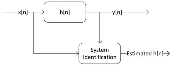
The model-free approach is shown in Figure 1. The model-free approach uses input and output data to synthesize the system model. The system parameters change with time because of different reasons such as component aging and lifetime issues. As a result, a system model derived using differential equations is unable to accommodate these changes. These factors have given rise to a model-free approach for developing the system models.

Figure 1.
Model-free approach.
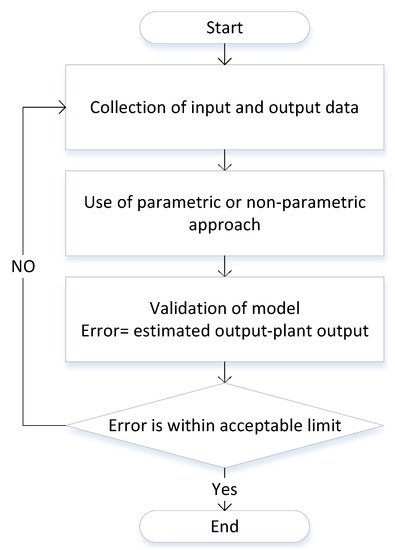
The process of the model-free approach is shown in Figure 2. The first step is the collection of the input and output data. Filtering is performed on these data to remove the noise. The second step is the use of a model-free approach for the estimation of the system model. Two major approaches for the model-free approach are parametric [1][15] and non-parametric [2][16] system identification. The third step is the validation of the estimated model. Model validation is performed by comparing the outputs of the estimated model with the actual plant outputs. If the difference in the outputs is within acceptable limits, then the estimated model is the required model. If the difference is not within acceptable limits, then the whole process of the model-free approach has to be repeated.

Figure 2.
Model-free approach process.
1.1. Non-Parametric Approach
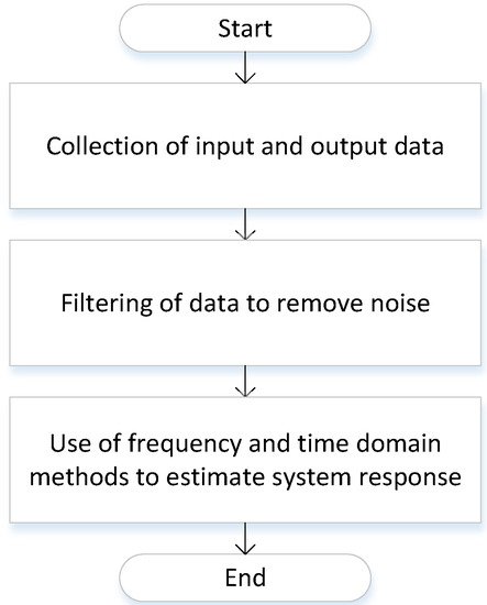
Non-parametric system identification uses frequency and time domain methods for measured input and output data for estimating the system response. Figure 3 shows the process of non-parametric system identification.

Figure 3.
Non-parametric approach.
The first step is the collection of the output data for all possible inputs. The second step is the filtering of the data to remove the unwanted noise. The third step is the use of frequency domain methods such as Bode plots or time domain methods such as impulse response to estimate the system response. There is no need for model selection and estimation of model parameters such as parametric system identification. This aspect makes the implementation of non-parametric system identification easy to implement compared to parametric system identification. However, the performance of the non-parametric approach is prone to noise. As a result, a large number of data samples is required, which makes its response time slow. As a result, it is not feasible for applications such as power electronic converters, where the response time should be fast for any change in the voltage or current.
1.2. Parametric Approach
In a parametric approach [3][17], there are two main steps to obtain the model of the system. These steps are the selection of the model and the estimation of the parameters of the model. The selection of the model of the system is not a straightforward task. A good choice is the model that captures the necessary dynamics of the system and, at the same time, does not require too many computations. The model can be linear or non-linear and of any order. The greater the order of the model, the greater the accuracy of the estimated model will be with the real plant dynamics. However, a large-order model will have more computational burden compared to a lower-order model.
H(s)=as+bcs2+ds+e
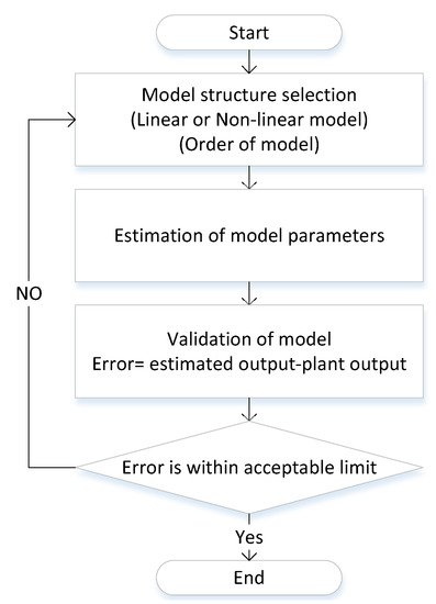
The process of the parametric approach is shown in Figure 4. The first step is to collect the input and corresponding output data. The second step is the selection of the model structure. The model can be linear or non-linear and of any order. The computational burden and accuracy of the estimated model depend on the order of the model. The greater the order of the model, the higher will be the accuracy of the estimated model and computational requirements. An ideal model is such that it captures the necessary dynamics of the system and does not require too many computations. After the selection of the model and its order, the third step is the estimation of the model parameters. As an example, take (16) as a system model. The parameters of this model are a, b, c, d, and e. Different algorithms have been proposed in the literature for the estimation of these parameters, such as the least-squares method. The next step is the validation of the estimated model by measuring an error. This error is the difference between the plant output and the estimated model output. If the error is within an acceptable range, then the estimated model is the correct choice. If the error is not within an acceptable range, then the whole process has to repeat for the estimation of the system model.

Figure 4.
Parametric approach.
2. Emerging Trends in Model-Free Predictive Control
2.1. Microgrids
Microgrids provide support to the main electric grid in case of any disturbance, and they are an option for providing electricity in areas where there is no access to electricity. Solar panels, wind turbines, and energy storage systems are some of the sources connected to the microgrid by using power electronic converters. Different control schemes have been proposed in the literature for microgrids [4][36]. The most widely used control scheme is the hierarchical control of the microgrid. This hierarchical control consists of three layers, known as primary, secondary, and tertiary. These layers are divided based on response time and bandwidth requirements for the communication. Table 1 6 shows the functions of different layers and their response time.
Table 16.
Hierarchical control layer functions and their response time.
| Layer | Function | Time Response | ||
|---|---|---|---|---|
| Primary |
| Fast | ||
| Secondary |
| Slow | ||
| Tertiary | Coordination of different microgrids | Slow |
Two main challenges in the control of microgrids are frequency [5][6][37,38] and voltage regulation. For frequency and voltage regulation, model-based controllers have been proposed. Among these model-based controllers, model predictive control (MPC) offers many advantages in microgrids because of its flexibility to include constraints and non-linearities in a systematic way [7][39]. However, the major drawback of the MPC is the model of the microgrid. Modern microgrids have complex dynamics, and they have a non-linear nature. Due to their complex nature, an explicit representation of the state variable is not possible. Moreover, solving these non-linear equations requires much computational effort. To solve this problem, reduced model or linearization methods are commonly used. However, the reduction in model or linearization compromises capturing the dynamics of the system. As a result, it affects the performance of the MPC. Due to these factors, model-free predictive control (MFPC) has gained attention in microgrids. There is much potential for MFPC in microgrids.
2.2. Model Reduction
For the non-parametric approach, two main components are the selection of a model structure and the identification of the model parameters. Applications such as power electronic converters have a non-linear nature. Approximating this non-linear behavior with a simple non-linear model is an active area of research [8][40]. Moreover, the approximation of non-linear models with a linear model is also an active area of research [8][40]. Model order reduction is an active research domain in the model-free approach. The reduction in the order of the model reduces the computational load of the controller.
2.3. Convexification
The estimation of model parameters is a major process in the model-free approach. Different estimation techniques have been proposed in the literature for the estimation of the model parameters. Convexification is the process of converting an estimation problem into a convex function. Computationally efficient schemes are available for finding the global minima of a convex function. Convexification [8][40] is also an active research area in the model-free approach.
