Light Field Image Super-Resolution

Light Field Image Super-Resolution: Comparison

Please note this is a comparison between Version 1 by Li Yu and Version 2 by Lindsay Dong.

Light fields play important roles in industry, including in 3D mapping, virtual reality and other fields. However, as a kind of high-latitude data, light field images are difficult to acquire and store. Compared with traditional 2D planar images, 4D light field images contain information from different angles in the scene, and thus the super-resolution of light field images needs to be performed not only in the spatial domain but also in the angular domain. In the early days of light field super-resolution research, many solutions for 2D image super-resolution, such as Gaussian models and sparse representations, were also used in light field super-resolution. With the development of deep learning, light field image super-resolution solutions based on deep-learning techniques are becoming increasingly common and are gradually replacing traditional methods. In this paper, the current research on super-resolution light field images, including traditional methods and deep-learning-based methods, are outlined and discussed separately.

light field
image super-resolution
deep learning
convolutional neural networks

1. Introduction

The eye can see objects in the world because it receives the light emitted or reflected by the object. The light field is a complete representation of the collection of light in the three-dimensional world. Therefore, collecting and displaying the light field can visually reproduce the real world to a certain extent. In 1846, Michael Faraday [1] proposed the idea of interpreting light as a field.

Gershun [2] introduced the concept of a “light field” in 1936 by representing the radiation of light in space as a three-dimensional vector of spatial positions. Adelson and Bergen [3] further refined the work of Gershu [2] in 1991, and they proposed the “Plenoptic Function”, which uses five dimensions to represent light in the three-dimensional world. Levoy [4] reduced the 5-dimensional Plenoptic function to four dimensions by fixing the intensity of the light during propagation, which is now called a 4D light field.

As shown in Figure 1, the model proposed by Levoy uses two planes to simultaneously record the angle and position information of light in the space.

L (u, v, s, t)

represents a sample of light field, where L represents the light intensity. The viewpoint plane

(u, v)

is located on the

Z = 0

plane and records the direction information of the light. The image plane

(s, t)

is parallel to the viewpoint plane and is located on the plane of the camera coordinate system

Z = f

, which records the position information of the light (f as the distance between the two planes). Any ray emitted from a point

(X, Y, Z)

in space can be uniquely determined by knowing its intersection with the viewpoint plane

(u, v)

and the image plane

(s, t)

/media/item_content/202207/62e09a2439ca3electronics-11-01904-g001.png

Figure 1.

The two-plane parametric representation of the four-dimensional light field.

As a kind of high-dimensional data, light field data is difficult to be formally expressed in the three-dimensional world. Therefore, the early collection of 4D light field images requires special light field cameras ^[5][6][5,6]. As shown in Figure 2, the light field camera embeds a micro lens array between the main lens of the traditional camera and the photosensor. Light going through the main lens will be projected onto the photosensor plane after passing through the micro lens units on the micro lens array to form a unit image.

Figure 2.

Schematic diagram of light field camera imaging.

If each unit image is regarded as a macro-pixel, the points at the same position of each macro-pixel correspond to samples of the same direction at different positions of the photographed object. The image array, generated by extracting the pixels at the same position in each macro-pixel, can form a sub-image array of different directions, i.e., sub-aperture image, which contains both angular and spatial information of the photographed object. These pixels can form a sub-aperture image together. These sub-aperture images are the images formed by each angle of the light field so that angle information and spatial information can be captured at the same time.

Although there are various methods of light field collection, the light field images collected by these methods have various problems. For example, although the micro lens array can form a light field image through a single shot, its spatial resolution and angular resolution are inadequate for generating a clear image; while the light field data acquired by encoding masks can improve the angular resolution without sacrificing the image resolution, the peak signal-to-noise ratio (PSNR) of its acquired data is low. In order to optimize the collected light field image, it is necessary to perform super-resolution processing ^[7][11]. Early light field super-resolution methods mainly include geometric projection ^[8][12] and optimization using prior knowledge. The projection is mainly based on the imaging principle of the light field camera, using rich sub-pixel information to propagate the pixels of each sub-aperture image to the target view for super-resolution. Nava ^[9][13] obtained inspiration from the Focal Stack transformation and developed a projection-based technology. The method based on optimization mainly relies on different mathematical models to perform super-resolution processing on a light field under various optimization frameworks. Bishop ^[10][14] performed this task by means of a variational Bayesian framework. With the boom in artificial intelligence in recent decades, deep learning has proven its effectiveness in many fields, including image super-resolution ^[11][15], image depth estimation ^[12][16], object detection ^[13][17], face recognition ^[14][15][16][18,19,20] and biometrics ^[17][21]. At the same time, deep learning is also used in the task of light field super-resolution. The method proposed by Yoon ^[18][22] laid a solid foundation for the combination of deep learning and light field super-resolution.

2. Traditional Method

2.1. Projection-Based LFSR

The spatial resolution of the sub-aperture image is limited by the microlens resolution. The geometric projection-based approach calculates sub-pixel offsets between sub-aperture images of different views, based on which pixels in adjacent views can be propagated to the target view for super-resolution processing of the target view. Lim ^[19][28] indicatedthat the angular data in the 2D dimension of the light field contains information about the sub-pixel offsets of images in the spatial dimension from different viewpoints. After extracting this information, the light field image can be super-resolution processed by projection onto convex sets (POCS) ^[20][29]. Nava ^[9][13] proposed a new super-resolution focus stack based on Fourier slice photographic transformation ^[21][30] and combined it with multi-view depth estimation to obtain super-resolution images. Pérez ^[22][31] extended the Fourier slicing technique to the super-resolution work of the light field and provided a new super-resolution algorithm based on Fourier slicing photography and discrete focus stack transform.

2.2. Priori-Knowledge Based LFSR

During the shooting process of the light field camera, due to the interference of external factors, such as the environment, light, and jitter, the obtained light field images often have low resolution and varying degrees of noise disturbance. In order to reconstruct a more realistic view with high resolution, a method based on a prior hypothesis was proposed. This type of method used the special high-dimensional structure of the 4D light field while adding priori assumptions about the actual shooting scene, and then proposed a mathematical model to optimize the solution of the super-resolution problem of the light field. Boominathan ^[23][41] used a low-resolution LF camera and a high-resolution digital single-lens reflex (DSLR) camera to form a hybrid imaging system and used a patch-based algorithm to combine the advantages of the two cameras to produce high-resolution images. The method proposed by Pendu ^[24][42] based on the Fourier parallax layer model ^[25][43] can simultaneously solve various types of degradation problems in a single optimization framework.

3. Deep-Learning-Based Method

The prosperous development of deep learning has promoted the development of image super-resolution. The super-resolution convolutional neural network (SRCNN) proposed by Dong ^[26][44] in 2014 represented the end-to-end mapping between low/high resolution images. As shown in Figure 34 below, in order to learn this mapping, only three steps are required: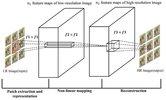

Figure 34. Pipeline of SRCNN ^[26].

Pipeline of SRCNN [44].

1.

Patch extraction and representation: This operation extracts patches from low-resolution images and expresses them as high-dimensional vectors. The dimensionality of the vector is equal to the number of feature maps.

2.

Non-linear mapping: This operation can non-linearly map the high-dimensional vector extracted in 1 to another high-dimensional vector, and each mapping vector can conceptually represent a high-resolution patch; these mapping vectors form another set of feature maps.

3.

Reconstruction: This operation will operate the high-resolution patch set obtained in Step 2 to generate the final high-resolution image.

This kind of lightweight network structure achieved state-of-the-art recovery quality at that time, which was the first combination of deep learning and image super-resolution work. The subsequent network models for image super-resolution processing, such as very deep super-resolution network (VDSR) ^[27][45] and enhanced deep super-resolution network (EDSR) ^[28][46] were also inspired by it. Although the good generalization ability of convolutional neural networks can provide enough training data to fit the model and cover a wide distribution of the expected test images, these super-resolution algorithms for single images cannot be directly applied to the super-resolution problem of light field images. Compared with the SISR work that only considers increasing the spatial resolution, the target of the light field super-resolution includes increading both the angular resolution and the spatial resolution. In 2015, Yoon ^[18][22] proposed a neural network model, which was named light field convolutional neural network (LFCNN), for light field image super-resolution, its overall structure is shown in Figure 45. The network model consists mainly of a spatial SR network and an angular SR network, with three different types of sub-aperture image pairs used as input throughout the network: horizontal pairs (

n = 2

), vertical pairs (

n = 2

) and surroundings (

n = 4

). The spatial SR network is similar to ^[29][47] and can restore the high-frequency details of the image. The angular SR network can generate new views between sub-aperture images, which is equivalent to increasing the number of sub-aperture images.

Figure 45. Overall framework of LFCNN ^[18].

Overall framework of LFCNN [22].

The special feature of LFCNN is that no matter how the depth and space of the scene change, the specific network layer used for angle and spatial resolution enhancement can restore the sub-aperture image well, thereby, improving the resolution of the image space domain and angular domain at the same time.

3.1. Sub-Aperture-Image-Based LFSR

3.1.1. Intra-Image-Similarity-Based LFSR

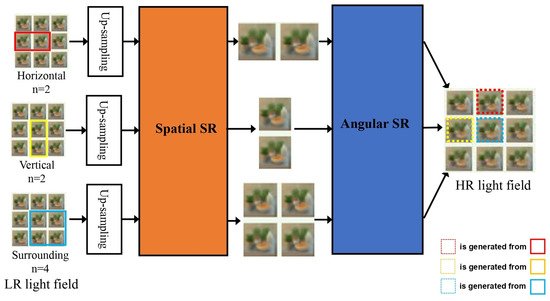
Early light field super-resolution methods based on deep learning usually divide different sub-tasks for processing, and the results of the sub-tasks work together to generate the final high-resolution light field image. As shown in Figure 57, the network model proposed in this period usually contains two network branches to process the angular domain and the spatial domain of the light field. The networks designed by Gul ^[30][52], Ko ^[31][60], and Jin ^[32][61] all follow this processing idea. Gul ^[30][52] used light field images with low angular resolution and low spatial resolution as the input of the network.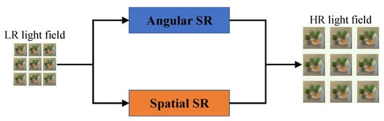

Figure 57.

Network model of light field super resolution with two sub-network branches.

First, through the angular SR network, a new sub-aperture image is synthesized by interpolation and the output has low spatial resolution and high angular resolution. The spatial SR network takes the output of the angular SR network as input, improves the spatial resolution of each sub-aperture image through training, and finally outputs a light field image with high spatial resolution and high angular resolution. The AFR module can perform feature remixing on the multi-view features extracted by the network through the disparity estimator according to the angular coordinates. The network can generate high-quality super-resolution images regardless of the angular coordinates of the input view images. The method proposed by Jin ^[32][61] used two sub-network modules to model the complementary information between views and the parallax structure of the light field image, while fusing the complementary information between views, the original parallax structure of the light field is preserved. In addition to processing the angular domain and the spatial domain of the light field separately, there are also some methods that treat the two as an interconnected whole. Yeung ^[33][62] used four-dimensional convolution to characterize the high-dimensional structure of the light field image and designed a special feature extraction layer that can extract the joint spatial and angular features on the light field image to perform super-resolution processing of the light field image.

3.1.2. Inter-Image-Similarity-Based LFSR

Ordinary image SR based on deep learning tends to exploit only the external phase between images, i.e., training the network with many image datasets, thus embedding the natural image prior into the neural network model. Although for general image SR, better super-resolution performance can be obtained by only using the external similarity of the image; however, this is not sufficient for processing complex light field SR. There is also a high degree of similarity between different angle views in the light field, i.e., the internal similarity of the light field. The internal similarity of the light field provides a wealth of information for super-resolution of each view. Therefore, comprehensive utilization of the internal and external similarities of the light field can greatly improve the performance of the learning-based light field SR. As shown in

Figure 6, Fan ^[34] divides the light field super-resolution processing into a two-stage task, using external similarity and internal similarity in the two stages of the task. In the first stage, the VDSR network is trained to use the external similarity to enhance the view, and in the second stage, the max-pooling convolutional neural network (MPCNN) is trained so that it can use the internal similarity to further enhance the target view from the information of the neighboring views.

9, Fan [53] divides the light field super-resolution processing into a two-stage task, using external similarity and internal similarity in the two stages of the task. In the first stage, the VDSR network is trained to use the external similarity to enhance the view, and in the second stage, the max-pooling convolutional neural network (MPCNN) is trained so that it can use the internal similarity to further enhance the target view from the information of the neighboring views.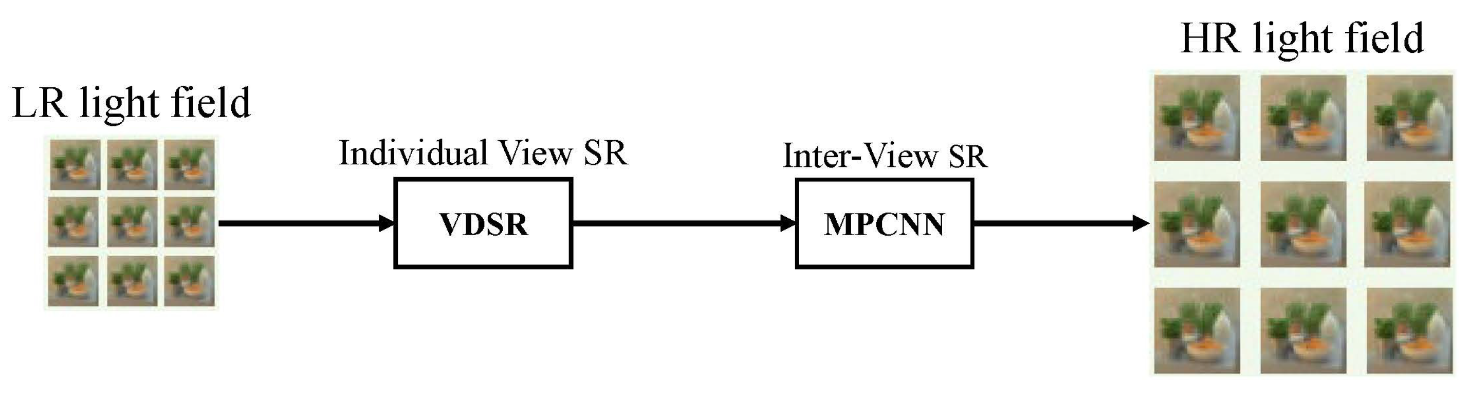

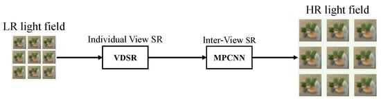/media/item_content/202207/62e09b32b5323electronics-11-01904-g009.png

Figure 69. Network structure proposed by Fan ^[34].

Network structure proposed by Fan [53].

3.2. Epipolar-Plane-Image-Based LFSR

EPI is a 2D slice of a 4D light field with a constant angle and spatial direction, which contains the depth information of the scene; therefore, it is usually used for the depth estimation of the light field; however, some researchers attempt to apply it to light field super-resolution tasks.

Wafa ^[35][80] designed an end-to-end deep-learning model to process all sub-aperture images at the same time, and used EPI information to smoothly generate views. Yuan ^[36][54] used EPI to restore the geometric consistency of light field images lost in SISR processing and proposed a network framework consisting of SISR deep CNN and EPI enhanced deep CNN. Inspired by the non-local attention mechanism ^[37][81], Wu ^[38][82] computed attention non-locally on the epipolar plane pixel by pixel, thus generating an attention map of the spatial dimension and guiding the reconstruction of the corresponding angular dimension based on the generated attention map.

4. Data Set and Comparison

4.1. Data Set

In chronological order, the current main light field data sets available for training and testing include: HCI old ^[39][49], STFlytro ^[40][83], EPFL ^[41][51], HCI ^[42][50], 30scenes ^[43][68]. Among them, HCI old, HCI, and 30scenes belong to the synthetic image data set, and the images of STFlytro and EPFL come from real-world images collected by a camera. The data set list is shown in Table 12.

Table 12.

Overview of the light field super-resolution data sets.

Data Set	Years	Number of Scenes	Shooting Method
HCI old ^[39]	HCI old [49]	2013	13	Blender Synthesis
STFlytro ^[40]	STFlytro [83]

23 shows the comparison between traditional method and deep-learning-based method. Traditional methods are mainly based on expert experience and prior knowledge, which can achieve better reconstruction quality at local details; however, the overall quality is sacrificed. Deep-learning-based methods can automatically reconstruct image by training network over huge amount of data, and the reconstructed image usually has a quality improvement at both local and global scale. In addition, compared with traditional methods, deep-learning-based method has faster processing speed when faced with a large batch of LSFR tasks.

Table 23.

Comparison of traditional methods and deep-learning-based methods for light field image super resolution.

	Traditional Method	Deep-Learning-Based Method
Reconstruction Quality	Good detail but poor overall quality	Good detail and overall quality
2016	9	Lytro Illum
Advantages	No training required. Process explainable.	Automatic feature extraction. Parallel processing.	EPFL ^[41]	EPFL [51]	2016	10	Lytro Illum
Disadvantages	Relying on expert experience. Weak generalization ability. Poor robustness.	High computational complexity. Relying on dataset.	HCI ^[42]	HCI [50]	2016	24	Blender Synthesis
30scenes ^[43]	30scenes [68]	2016	30	CNN Synthesis

4.2. Comparison

Table

As for performance, several traditional and deep-learning-based LFSR works are selected for comparison, as shown in Table 34. The $\times 2$ SR ratio is chosen. PSNR and SSIM are evaluation metrics.

Table 34. Performance comparison of light field super-resolution algorithms, where best results are in bold and “-” means not tested. The five methods above are traditional methods, while others are deep learning based methods.

	HCI Old (PSNR/SSIM)	HCI (PSNR/SSIM)	EPFL (PSNR/SSIM)	STF Lytro (PSNR/SSIM)
Method	HCI Old (PSNR/SSIM)	HCI (PSNR/SSIM)	EPFL (PSNR/SSIM)	STF Lytro (PSNR/SSIM)
Mitra ^[44]	Mitra [35]		29.60/0.899	-	-	25.70/0.724
Wanner ^[45]	Wanner [48]		30.22/0.901	-	-	-
Wang ^[46]	Wang [34]		35.14/0.951	-	-	-
farrugia ^[47]	farrugia [40]		30.57/-	-	-	32.13/-
Pendu ^[24]	Pendu [42]		38.64/-	36.77/-	-	-
Yoon ^[18]	Yoon [22]		37.47/0.974	-	-	29.50/0.796
Wang ^[48]	Wang [23]		36.46/0.964	33.63/0.932	32.70/0.935	30.31/0.815
Zhang ^[49]	Zhang [24]		41.09/0.988	36.45/0.979	35.48/0.973	-
Kim ^[27]	Kim [45]		40.34/0.985	34.37/0.956	32.01/0.959	29.99/0.803
Ko ^[31]	Ko [60]		42.06/0.989	37.21/0.977	36.00/0.982	-
Jin ^[32]	Jin [61]		-	38.52/0.959	-	41.96/0.979
Yeung ^[33]	Yeung [62]		-	-	-	40.50/0.977
Wang ^[50]	Wang [57]		44.65/0.995	37.20/0.976	34.76/0.976	38.81/0.983
Zhang ^[51]	Zhang [66]		42.14/0.981	37.01/0.963	35.81/0.961	-
Fan ^[34]	Fan [53]		40.77/0.968	-	-	-
Cheng ^[52]	Cheng [70]		36.10/-	-	30.41/-	-
Ma ^[53]	Ma [58]		43.90/0.993	40.49/0.986	41.38/0.989	-
Jin ^[54]	Jin [73]		-	-	-	34.39/0.951
Cheng ^[55]	Cheng [59]		40.03/-	37.94/-	34.78/-	38.05/-
Ribeiro ^[56]	Ribeiro [69]		45.49/0.964	38.22/0.956	34.41/0.953	-
Farrugia ^[57]	Farrugia [75]		-	-	-	32.41/0.884
Meng ^[58]	Meng [56]		-	32.45/-	34.20/-	-
Wu ^[59]	Wu [27]		-	-	-	42.48/-
Zhu ^[60]	Zhu [55]		-	-	-	33.04/0.958
Wafa ^[35]	Wafa [80]		39.76/0.968	-	-	44.45/0.995
Yuan ^[36]	Yuan [54]		38.63/0.954	-	-	40.61/0.984
Meng ^[61]	Meng [77]		33.12/0.913	34.64/0.933	35.97/0.947	38.30/0.969
Kim ^[62]	Kim [67]		-	-	-	39.25/0.990
Jin ^[63]	Jin [74]		41.80/0.974	37.14/0.966	-	-