Your browser does not fully support modern features. Please upgrade for a smoother experience.
Please note this is a comparison between Version 1 by Joao Manuel R.S. Tavares and Version 2 by Vivi Li.
The crowd counting task has become a pillar for crowd control as it provides information concerning the number of people in a scene. It is helpful in many scenarios such as video surveillance, public safety, and future event planning. To solve such tasks, researchers have proposed different solutions. In the beginning, researchers went with more traditional solutions, twhenile recently the focus is on deep learning methods and, more specifically, on Convolutional Neural Networks (CNNs), because of their efficiency.
- computer vision
- deep learning
- people counting
- sparse datasets
- crowded datasets
1. Background
Because of the fast growth of the world’s population, and situations where crowds occur, such as concerts, political speeches, rallies, marathons, and stadiums, crowd counting is becoming an active research topic in computer vision [1]. The task of crowd counting, defined as determining the number of people in a crowd, would help in many fields, such as in video surveillance for safety reasons, human behavior analysis, and urban planning [2][3][4][5][2,3,4,5]. Many approaches have been proposed in the literature to solve this problem, which generally can be split into four categories: detection, regression, density estimation, and approaches based on convolutional neural networks (CNNs).
2. Introduction
As mentioned previously, this rentryview divides the crowd counting models into four categories. Starting with the detection-based method, the principle behind it to use a moving window as a detector to identify and count how many persons are in an input image [6]. Although these methods work well for detecting faces, they do not perform sufficiently well on crowded images as most target objects are not clearly visible. Counting by detection is categorized into five types: monolithic detection [7][8][9][7,8,9], part-based detection [10][11][10,11], shape matching [12][13][12,13], multi-sensor detection [14], and transfer learning [15][16][15,16]. Since counting by detection is not very precise when factors such as dense crowds and high background clutter appear, researchers proposed a regression method [17] to overcome these problems, where neither segmentation nor tracking individuals are involved. First, it extracts the low-level features such as edge details and foreground pixels and then applies regression modelling to them by mapping the features and the count. Clustering models are about selecting and gathering feature points or trajectories of feature points. These methods use unsupervised learning to identify each moving entity by an independent motion [18]. Among existing approaches, CNN based methods [19][20][19,20] have proved their efficiency and exhibit the best results for the crowd counting task. The general concept behind using deep convolutional networks is to scan the input image to understand its different features and then to combine the different scanned local features to classify it. According to the used network architecture, crowd counting models can be classified into: basic CNN [21][22][21,22], multi-column [23][24][25][23,24,25], and single column-based methods [26][27][28][29][30][26,27,28,29,30].3. Heuristic Models
Early methods of this category estimate the pedestrian number via heuristic methods [31], for instance detection-based, regression-based, and density-estimation-based methods. This section explains in more detail these models and how they work.3.1. Detection Based Methods
Earlier works on crowd counting were focused on detection-based methods to determine the number of people in the crowd [32][33][34][32,33,34]. They mainly detect each target person in a given image using specific detectors. In the following paragraphs, an explanation of these methods with some examples is given. Monolithic detection: it is considered a typical pedestrian detection approach that trains the classifier, utilizing the entire body of a set of pedestrian training images [7][8][9][31][7,8,9,31]. In order to represent the entire body’s appearance, common features are used: Haar wavelets, gradient-based features, edgelet, and shapelets. As to the classification, several classifiers were used:-
Non-Linear: Similarly to RBF, Support Vector Machines (SVMs) present good quality while suffering from low detection speed.
3.2. Regression Methods
Because of the difficulty of detection-based models in dealing with highly dense crowds and high background clutter, researchers introduced regression-based approaches, which are inspired by the capacity of humans to determine the density at first sight without the need to enumerate how many pedestrians are in the scene under analysis [17]. Such a method counts people in crowded scenes by discovering a direct mapping from low-level imagery features to crowd density. First, it extracts global features [38]: texture [39], gradient or edge, or local features [40], such as Scale-invariant Feature Transform (SIFT), Local Binary Patterns (LBP), Histogram of Oriented Gradients (HOG), and Gray Level Co-occurrence Matrix (GLCM). After the feature extraction step, it trains a regression model to indicate the count given the normalized features. Among the regression techniques, one can mention: linear regression [41], piecewise linear regression [17], and Gaussian mixture regression [42]. Another approach from Idrees et al. [43] considered that, in highly crowded scenes, there is no feature or detection approach reliable enough to deliver sufficient information for a precise counting because of the low resolution, severe occlusion, foreshortening, and perspective problems. Furthermore, the presence of a spatial relationship is used in constraining the count estimates in neighboring local regions, and it is suggested that the extraction of features be performed using different methods to catch the different information. Table 1 summarizes some of the regression-based methods.Table 1.
Summary of regression-based methods.
| Method | Global Features | Regression Model | Dataset(s) | |||
|---|---|---|---|---|---|---|
| [44] | Segment, internal edge, texture | Gaussian | Peds1, Peds2 | |||
|
|
[45] | Segment, motion | |||
| Pooling layer | Linear regression |
| PETS2009 | |||
|
|
[46] | Segment, edge, gradient | Gaussian | UCSD pedestrian, Pets 2009 | |
| [38] | Segment, edge, texture | Kernel ridge regression | UCSD, Mall | |||
| [47] | Edge | Linear regression | Internal data (2000 images, number of people per image: from 3 to 27 people) |
3.3. Clustering Based Methods
Another alternative technique is counting by clustering. The idea is to decompose the crowd into individual entities. Each entity has unique patterns that can be clustered to determine the number of individuals [31]. Rabaud et al. [48], used a simple yet effective tracker, the Kanade–Lucas–Tomasi (KLT), to extract a large set of low-level features in pedestrian videos. It is proposed as a conditioning technique for feature trajectories to identify the number of objects in a scene. A complementary trajectory set clustering method was also introduced. The method can only be applied to crowd-counting videos. Three different real-world datasets were used to validate and determine the method’s robustness: USC, Library, and Cells datasets [49]. Brostow et al. [50], proposed a simple unsupervised Bayesian clustering framework to capture people in moving gatherings, the principal idea being to track local features and group them into clusters. The algorithm tracks simple image features and groups them into clusters defining independently-moving entities in a probabilistic way. The method uses space-time proximity and trajectory coherence via image space as the only probabilistic criteria for clustering. This solution came instead of determining the number of clusters and setting constituent features with supervised learning or a subject-specific model. The results were encouraging from crowded videos of bees, ants, penguins, and most humans. Rao et al. [51], explained the importance of crowd density estimation in a video scene to understand crowd behavior by implementing a crowd density estimation method based on clustering motion cues and hierarchical clustering. For motion estimation, the approach integrates optical flow. It employs contour analysis to detect crowd silhouettes and clustering to calculate crowd density. It starts by applying a lens correction profile to each image frame, followed by pre-processing the frames to remove noise. A Gaussian filter is applied to suppress high amplitude edges. Finally, the foreground pixels are mapped to crowd density by clustering the motion cues hierarchically. For evaluation, three datasets were used: MCG, PETS, and UCSD. Antonini et al. [52], worked on video sequences to improve the automatic counting of pedestrians. A generative probabilistic approach was applied to better represent the data. The main goal was to analyze the computed trajectories, find a better representation in the Independent Component Analysis (ICA) transformed domain, and apply clustering techniques to improve the estimation of the actual count of pedestrians in the scene. The advantage of using the ICA generative statistical model is in reducing the influence of outliers.4. Deep Learning Methods
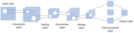
Because of the CNN architecture’s efficiency in many tasks, including crowd counting, recent researchers used CNN as the base framework of their work. The general concept is to understand the various features of the image under analysis by browsing its content from left to right or top to bottom, and then combining the different scanned local features in order to classify it. A CNN includes three layers: convolutional layer, pooling layer, and fully connected layer [53][54][55][53,54,55]. Table 2 details each usual CNN layer with its actions, parameters, inputs and outputs.Table 2.
Details of the three CNN layers.
| Actions | Parameters | Input | Output | |
|---|---|---|---|---|
| Convolutional layer |
|
|
|
|
|
|
|
4.1. Basic CNN
Among the CNN architectures, one has the basic CNN with its light network. It adopts the primary CNN layers: the convolutional layer, the pooling layer, and the fully connected layer. Figure 24 presents a simplified structure of the fundamental CNN.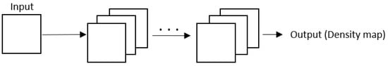
Figure 24.
General structure of the Basic CNN architecture.
-
Optimizing the connections: the multi-stage ConvNet increases the number of features in the final classifier, and the connections seriously increase the calculation time during the training and detection phases. Some redundant connections among two similar feature maps were observed, so these extra connections were removed based on a similarity matrix to accelerate the speed.
-
Cascade classifier: samples with complicated backgrounds are always hard to classify. The idea is to pick out those complex samples and train them individually and, after that, send them to a second ConvNet classifier to obtain the final classification result.
| ||||
|
|
|||
| Fully connected layer |
|
|
|
|
-
Convolutional layer: the primary role of this layer is to apply filters to detect features in the input image and build numerous feature maps to help identify or classify it. After every convolution operation, a linear function, the ReLU activation, is applied to replace the negative pixel values with zero values in the feature map.
-
Pooling layer: this step takes the output feature map generated by the convolution. The goal is to reduce the complexity for further layers by applying a specific function such as the max pooling.
-
Fully connected layer: every neuron from the previous layer is connected to every neuron on the next layer to generate the final classification result.
| |||
|
4.2. Multi column CNN
To solve the variation problem, researchers have resorted to a multi-column architecture. Despite being harder to train, it proved its efficiency in specific situations. It consists of using more than one column to catch multi-scale information. Figure 35 represents the overall architecture of the multi-column CNN.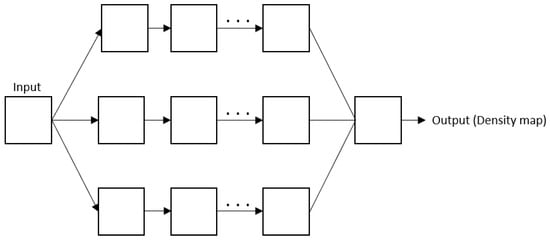
Figure 35.
Overall architecture of the multi-column CNN.