Watershed is a widely used image segmentation algorithm. A grayscale image is considered as topographic relief, which is flooded from initial basins. However, frequently they are not aware of the options of the algorithm and the peculiarities of its realizations. There are many watershed implementations in software packages and products. Even if these packages are based on the identical algorithm–watershed by flooding, their outcomes, processing speed, and consumed memory, vary greatly.
- segmentation
- watershed algorithm
- waterline
- flooding
1. Introduction
2. Description of Watershed Algorithms Applied in Software
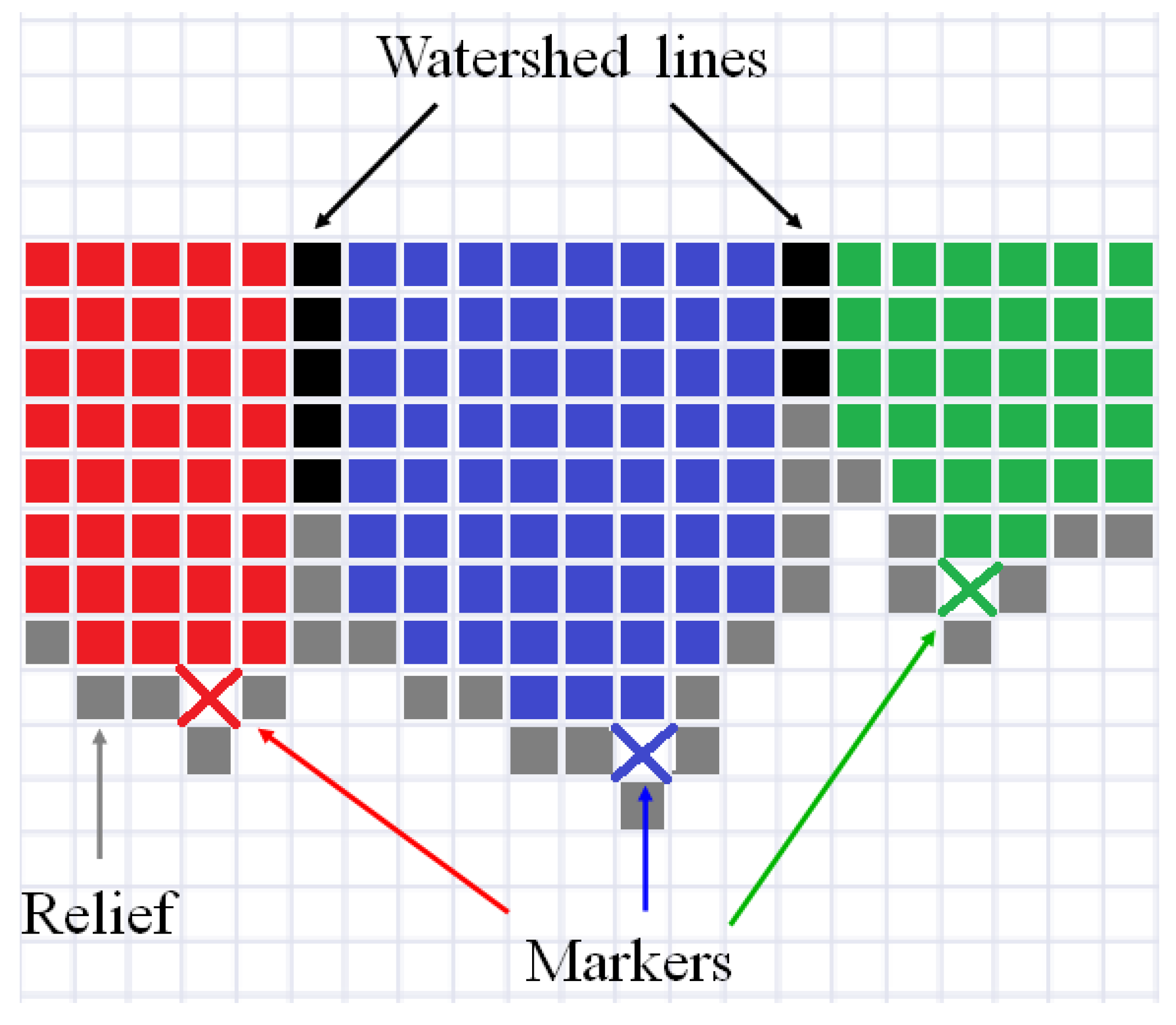
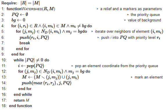
Because the considered algorithms are intended for processing both 2D and 3D images (strictly speaking, n-dimensional images can be processed), scholars use the term “image element” together with the terms pixel and voxel. Beucher and Lantuéjoul [5] introduced watershed for segmentation of grayscale images, although the watershed transformation as an operation of mathematical morphology was described a few years earlier [6][7]. To solve the oversegmentation problem caused by a huge number of initial basins started from each local minima of an image marker-controlled (or seeded) watershed was proposed [8]. Vincent and Soille [9] generalized watershed for an n-dimensional image and depicted an algorithm based on an immersion process analogy, in which the flooding of relief by water is simulated using a queue (first-in-first-out (FIFO) data structure) of image elements. Beucher and Meyer [10] developed effective algorithms, in which a flooding process is simulated by using a priority queue [11], where a priority is a value of a relief element, and a lower value corresponds to a higher priority. An illustrative example of a pseudocode describing steps of marker-controlled watershed by Beucher and Meyer is reported in Algorithm 1. Here, the variables and steps of this algorithm are explained: BM1 Image (relief) elements corresponding to markers (labels) that have at least one unmarked neighbor (i.e., marker of background ) are added to the priority queue ; see lines 4–9 in Algorithm 1. BM2 Element with the highest priority is extracted from the queue; if the priority queue is empty, then the algorithm terminates; see lines 10–11. BM3 Marker of the extracted element propagates on its unmarked neighbors; see lines 12–13. BM4 The neighbors marked in the previous step are inserted into the priority queue with the same priority or lower than the extracted element (if neighbor has higher relief value); then, go to step BM2; see line 14.| Algorithm 1 The marker-controlled watershed by Beucher and Meyer [10]. |
 |
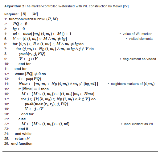
One can see that the algorithm by Beucher and Meyer does not form WL. Frequently, watershed lines are valuable segmentation outputs. Meyer [12] described the algorithm with WL construction. Pseudocode of this method is presented in Algorithm 2.
| Algorithm 2 The marker-controlled watershed with WL construction by Meyer [12]. |
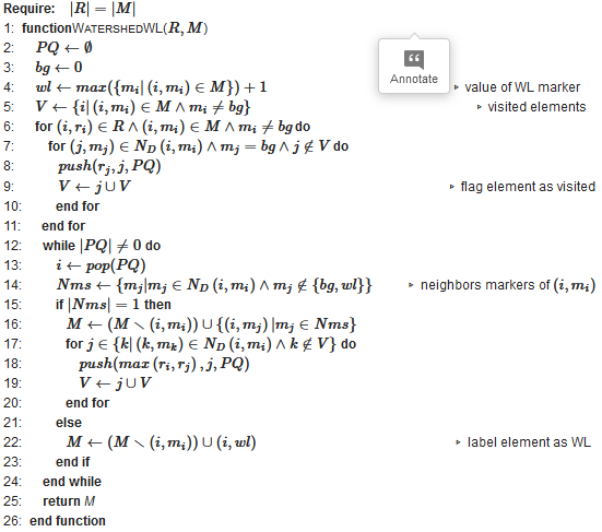 |
The variables and steps of the algorithm by Meyer are the following:
M1 Image elements corresponding to markers are flagged as visited ; see line 5 in Algorithm 2.
M2 Image elements having marked neighbors are added to the priority queue and flagged as visited; see lines 6–11.
M3 The element with the highest priority is extracted from the queue; if the priority queue is empty, then the algorithm terminates; see lines 12–13.
M4 If all marked neighbors of the extracted element have the same marker, then the image element is labeled by that marker; if marked neighbors of the extracted element have different markers, then the elements are flagged as WL-belonged with marker wl; see lines 14–23.
M5 Nonflagged as visited neighbors of the extracted element are added to a priority queue (with same or lower priority) and flagged as visited if the extracted element is not WL-belonged; then, go to step M3; see lines 17–20.
Paper [13] presents source codes of Algorithms 1 and 2 for processing 3D images with 26-connectivity in the Python programming language.
Scholars consider how to operate the above described marked-controlled algorithms with WL [12] and without WL [10] construction. Figure 2a shows a binary image containing two overlapping discs. Scholars generated this image by a simple code in Python. Then, scholars create a relief by subtracting a constant from a rectangular area in the center part of the inverted Euclidean distance transform (EDT) result for image containing two overlapping disks (see Figure 2b). The image containing initial markers (red and blue) is generated by placing the red and blue squares in the centers of the discs (Figure 2c); correspondingly, the markers are located in local minima of the relief. Segmentation results obtained by algorithms with (Figure 2e) and without WL (Figure 2d) construction are different. This example refutes the common misconception that differences in outcomes of watershed with and without WL result only from image elements of WL. The example clearly shows that segmentation results can vary.
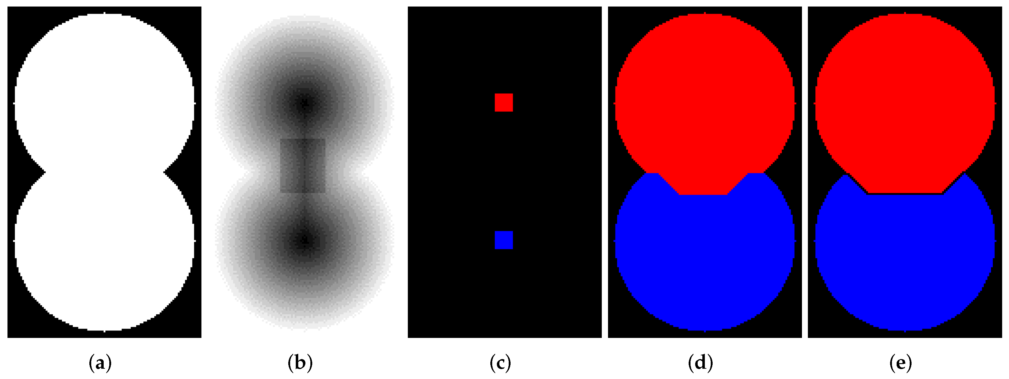
Figure 2. (a) Two overlapping binary discs; (b) relief; (c) initial markers; (d) segmentation result without watershed lines (WL) construction; (e) segmentation result with WL construction.
Although all flooding-based implementations have estimation of computational complexity as O(N), where N is the number of image elements, its processing speed strongly depends on the used data structures, applied programming language, software optimizations, asymptotic constant, and other parameters [14]. Hendriks [15] performed research on various priority queues in terms of performance and demonstrated the importance of selecting the appropriate priority queue realization. For digital elevation models (DEM) used in geographic information systems (GIS), Barnes et al. [16] showed how the choice of different queues affects a performance of flooding-based watershed algorithms.
Over the 30-year history of the watershed, many algorithms have been developed: by topographic distance [17], via image foresting transform [18][19], rain falling [20][21],
toboggan-based [22], via minimum spanning forest [23][24], hierarchical watersheds [25], etc. Surveys [26][27][28] compare various approaches for a watershed calculation. However, despite the enormous efforts to formulate the various mathematical concepts of watershed, only flooding-based algorithms are implemented in well-known software libraries.
Even if these packages are based on the identical algorithm, their outcomes, processing speed, and consumed memory, vary greatly. Papers [29][13] contain comprehensive benchmarking of various marker-controlled watershed implementations in software libraries and products.
References
- Bernardini, M.; Mayer, L.; Reed, D.; Feldmann, R. Predicting dark matter halo formation in N-body simulations with deep regression networks. Mon. Not. R. Astron. Soc. 2020, 496, 5116–5125.
- Negahbani, F.; Sabzi, R.; Jahromi, B.P.; Firouzabadi, D.; Movahedi, F.; Shirazi, M.K.; Majidi, S.; Dehghanian, A. PathoNet introduced as a deep neural network backend for evaluation of Ki-67 and tumor-infiltrating lymphocytes in breast cancer. Sci.Rep. 2021, 11, 8489.
- Kucharski, A.; Fabijanska, A. CNN-watershed: A watershed transform with predicted markers for corneal endothelium image segmentation. Biomed. Signal Process. Control 2021, 68, 102805.
- Gonzalez, R.C.; Woods, R.E. Digital Image Processing; Prentice Hall: Upper Saddle River, NJ, USA, 2008.
- Beucher, S.; Lantuéjoul, C. Use of Watersheds in Contour Detection. In Proceedings of the International Workshop on Image Processing: Real-Time Edge and Motion Detection/Estimation, Rennes, France, 17–21 September 1979; Volume 132.
- Lantuéjoul, C. La Squelettisation et son Application aux Mesures Topologiques des Mosa¨ıques Polycristallines. Ph.D. Thesis, Ecole des Mines, Paris, France, 1978.
- Digabel, H.; Lantuéjoul, C. Iterative algorithms. In Proceedings of the Actes du Second Symposium Européen d’Analyse Quantitative des Microstructures en Sciences des Matériaux, Biologie et Médecine, Caen, France, 4–7 October 1977; Chermant, J.L., Ed.; Dr. Riederer: Stuttgart, Germany, 1978; pp. 85–99.
- Meyer, F.; Beucher, S. Morphological segmentation. J. Vis. Commun. Image Represent. 1990, 1, 21–46.
- Vincent, L.; Soille, P. Watersheds in digital spaces: An efficient algorithm based on immersion simulations. IEEE Trans. Pattern Anal. Mach. Intell. 1991, 13, 583–598.
- Beucher, S.; Meyer, F. The morphological approach to segmentation: The watershed transformation. In Mathematical Morphology in Image Processing; Marcel Dekker, Inc.: New York, NY, USA, 1993; Volume 34, Chapter 12, pp. 452–464.
- Cormen, T.H.; Leiserson, C.E.; Rivest, R.L.; Stein, C. Introduction to Algorithms; MIT Press: Cambridge, MA, USA, 2009.
- Meyer, F. Un algorithme optimal de ligne de partage des eaux. In Proceedings of the 8th Congress AFCET, Lyon, France, 25–20 November 1991; Volume 2, pp. 847–859.
- Kornilov A, Safonov I, Yakimchuk I. A Review of Watershed Implementations for Segmentation of Volumetric Images. Journal of Imaging. 2022; 8(5):127.
- Kriegel, H.P.; Schubert, E.; Zimek, A. The (black) art of runtime evaluation: Are we comparing algorithms or implementations? Knowl. Inf. Syst. 2017, 52, 341–378.
- Hendriks, C.L.L. Revisiting priority queues for image analysis. Pattern Recognit. 2010, 43, 3003–3012.
- Barnes, R.; Lehman, C.; Mulla, D. Priority-flood: An optimal depression-filling and watershed-labeling algorithm for digital elevation models. Comput. Geosci. 2014, 62, 117–127.
- Meyer, F. Topographic distance and watershed lines. Signal Process. 1994, 38, 113–125.
- Lotufo, R.; Falcao, A. The Ordered Queue and the Optimality of the Watershed Approaches. In Mathematical Morphology and Its Applications to Image and Signal Processing; Goutsias, J., Vincent, L., Bloomberg, D.S., Eds.; Springer: Boston, MA, USA, 2000; pp. 341–350.
- Falcão, A.X.; Stolfi, J.; de Alencar Lotufo, R. The image foresting transform: Theory, algorithms, and applications. IEEE Trans. Pattern Anal. Mach. Intell. 2004, 26, 19–29.
- Bieniek, A.; Moga, A. An efficient watershed algorithm based on connected components. Pattern Recognit. 2000, 33, 907–916.
- De Smet, P.; Pires, R. Implementation and analysis of an optimized rainfalling watershed algorithm. In Proceedings of the Image and Video Communications and Processing, San Jose, CA, USA, 25–28 January 2000; Volume 3974, pp. 759–766.
- Lin, Y.C.; Tsai, Y.P.; Hung, Y.P.; Shih, Z.C. Comparison between immersion-based and toboggan-based watershed image segmentation. IEEE Trans. Image Process. 2006, 15, 632–640.
- Meyer, F. Minimum Spanning Forests for Morphological Segmentation. In Mathematical Morphology and Its Applications to Image Processing; Serra, J., Soille, P., Eds.; Springer: Dordrecht, The Netherlands, 1994; pp. 77–84.
- Cousty, J.; Bertrand, G.; Najman, L.; Couprie, M. Watershed cuts: Minimum spanning forests and the drop of water principle. IEEE Trans. Pattern Anal. Mach. Intell. 2008, 31, 1362–1374.
- Perret, B.; Cousty, J.; Guimaraes, S.J.F.; Maia, D.S. Evaluation of hierarchical watersheds. IEEE Trans. Image Process. 2017, 27, 1676–1688.
- Mahmoudi, R.; Akil, M. Analyses of the watershed transform. Int. J. Image Process. 2011, 5, 521–541.
- Roerdink, J.B.; Meijster, A. TheWatershed Transform: Definitions, Algorithms and Parallelization Strategies. Fundam. Inf. 2000, 41, 187–228.
- Audigier, R.; de Alencar Lotufo, R. Watershed by image foresting transform, tie-zone, and theoretical relationships with other watershed definitions. In Proceedings of the 8th International Symposium on Mathematical Morphology, Rio de Janeiro, Brazil, 2007; Volume 1, pp. 277–288.
- Kornilov, A.S.; Safonov, I.V. An overview of watershed algorithm implementations in open source libraries. J. Imaging 2018, 4, 123.