The color analysis of sediment in the laboratory has followed important technological developments in closely related fields, such as the analysis of soils and sedimentary rocks, as well as in more distant fields, such as remote sensing. This has led to the development of sensors allowing the analysis of color and, more generally, of the electromagnetic spectrum of light to answer problems of rapidity, high resolution, automation, and increasing the amount of interesting information remotely without affecting the sample. The hyperspectral imaging sensor will be the focus of this practical guide.
- hyperspectral imaging
- image processing
- spectroscopy
- sediment core
1. Introduction
The focus is on the different steps that led to the use of hyperspectral imaging in the geosciences, the different fields involved in these developments, and their exploitation (Figure 1).
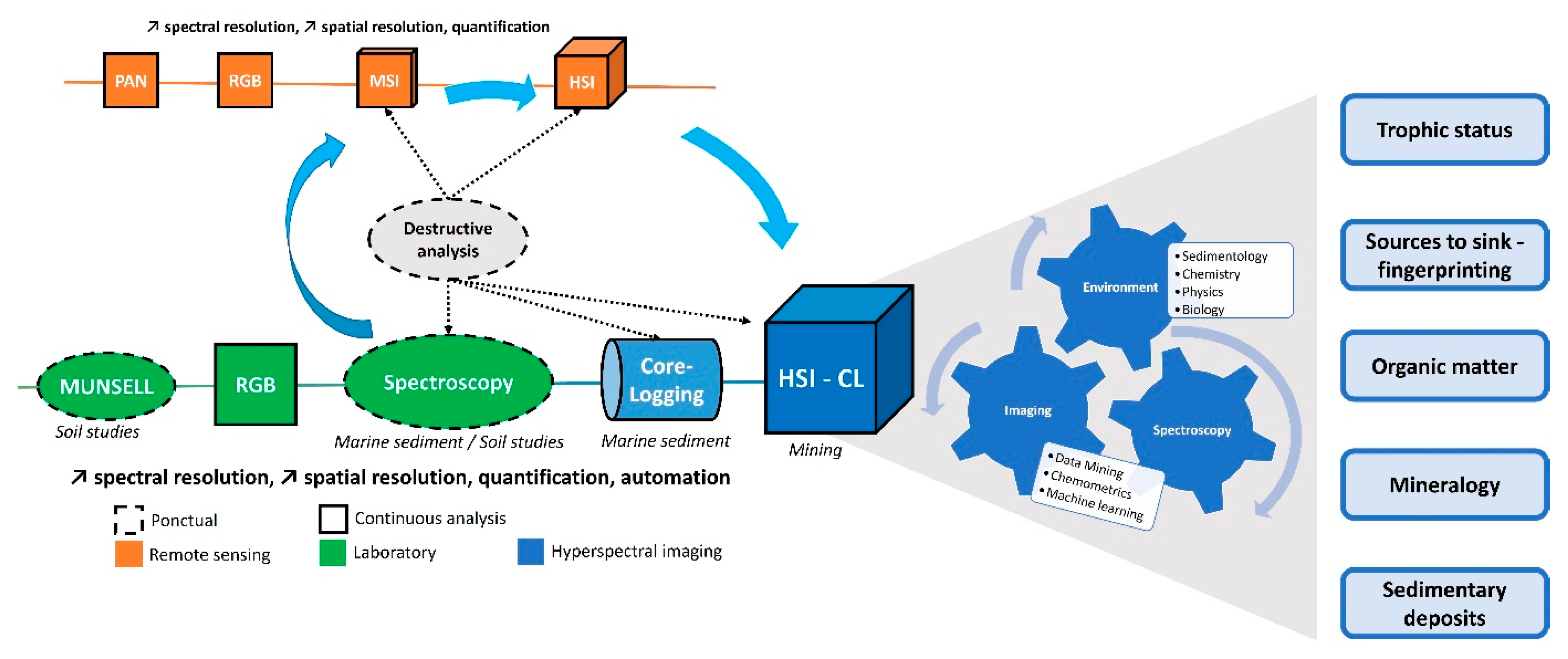
Figure 1. Schematic representation of the different techniques and domains involved in the development and exploitation of hyperspectral data for sediment core analysis (PAN: Panchromatic, MSI: MultiSpectral Image, HSI: HyperSpectral Image, CL: Core Logging) and some potential topics.
2. Munsell Lithology Description
3. RGB (Red, Green, Blue) Imaging
4. Spectroscopic Analysis
5. Hyperspectral Imaging
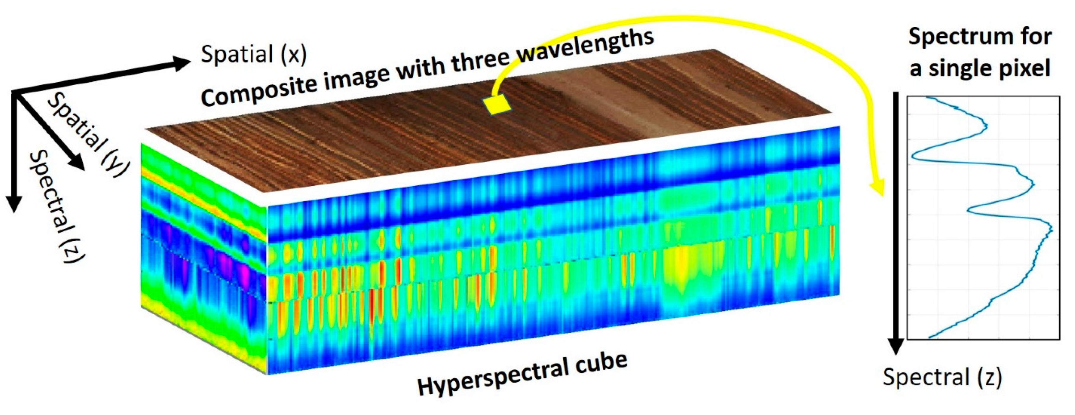 Figure 3. Hyperspectral cube composed of two spatial dimensions (x along and y across the sample, which can also be viewed as time and cross-time dimensions) and one spectral dimension (z as wavelengths, wavenumbers, or energies). Each pixel contains a spectrum, and wavelength assemblage can create a composite image.
5.1. Hyperspectral Sensors
5.2. Acquisitions and Recommendations
5.3. How to Process These Data?
To identify sedimentary processes recorded by hyperspectral data, four main steps are to be followed, fully or in part, as shown in Figure 4 [65] . (1) The first is to prepare the data by reducing the image to the spatial and spectral areas and to use pre-processing to reduce the noise present in the data. (2) The second allows to observe the first trends in the HSI, both in the spectral dimension with absorptions of some compounds and in the spatial dimensions with sedimentary deposits. (3) Data processing methods will allow to extract these first observations and to highlight other properties of interest with machine learning approaches. (4) The maps extracted by these methods can be spatially postprocessed to reduce the residual noise or to match the observations with other analyses. This last step can help to confirm the observations and to obtain an interpretation of the biophysical-chemical properties recorded by the hyperspectral sensors.
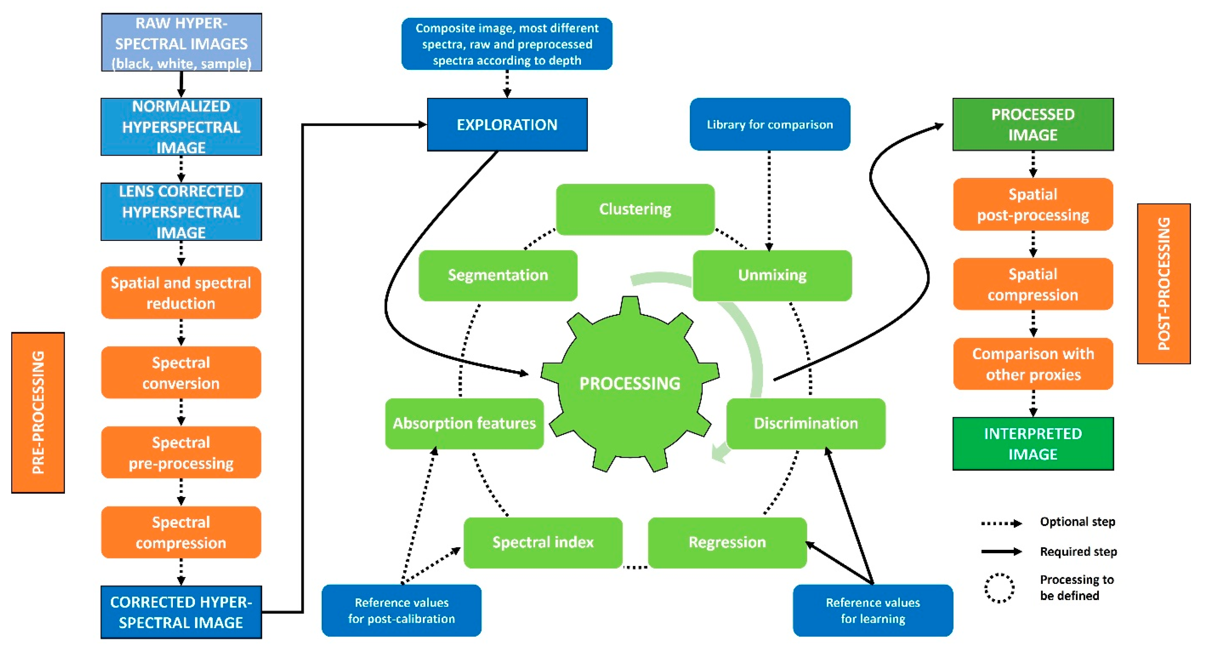 Figure 4. Diagram of the different steps that can be performed to (1) correct the initial HSI (prepro-cessing), (2) visualize the information contained in the image (exploration), (3) extract the information of interest (processing), and (4) apply a final correction (postprocessing) leading to a properly interpreted image.
5.4. What Sedimentary Properties Can Be Derived from It?
Five major themes aim to reveal the various sedimentary properties with the use of HSI and versatile methods. (1) The trophic status of lakes is extensively studied by spectroscopy, and HSI can take advantage of this work by leveraging specific pigment indices. (2) Source-to-sink studies can also be performed using spectral fingerprints (endmembers EMs) associated with sources in the lake catchment. (3) Organic matter is an important sediment property for paleoenvironmental reconstructions or the estimation of anthropogenic pollution and is generally characterized with regression/classification approaches or index definitions. (4) Sediment mineralogy is also an important property used to describe the sources of sediment supply within the watershed, and it can be characterized with indices or regression and classification methods. (5) Sedimentary structures and texture will have spectral and/or spatial fingerprints that can be recorded by HSI and characterized with classification methods. Another recent hyperspectral imaging review by Zander et al. focuses on the biogeochemical analysis of sediment cores and is complementary to the above [66].
References
- Munsell, A.H. A Color Notation; G.H. Ellis Company: Indianapolis, IN, USA, 1905.
- Hollister, C.D.; Heezen, B.C. Geologic Effects of Ocean Bottom Currents: Western North Atlantic. In Studies in Physical Oceanography; Gordon and Breach Science Publishers: Langhorne, PA, USA, 1972; pp. 37–66. ISBN 9780677151700.
- Ericson, D.B.; Ewing, M.; Wollin, G.; Heezen, B.C. Atlantic Deep-Sea Sediment Cores. Geol. Soc. Am. Bull. 1961, 72, 193–286.
- CIE. Colorimetry—Part 4: CIE 1976 L*a*b* Colour Space; CIE: Vienna, Austria, 2008.
- Miall, A.D. Principles of Sedimentary Basin Analysis; Springer: New York, NY, USA, 1984; ISBN 978-0-387-90941-7.
- Balsam, W.L.; Deaton, B.C.; Damuth, J.E. Evaluating Optical Lightness as a Proxy for Carbonate Content in Marine Sediment Cores. Mar. Geol. 1999, 161, 141–153.
- Bond, G.; Broecker, W.; Lotti, R.; McManus, J. Abrupt Color Changes in Isotope Stage 5 in North Atlantic Deep Sea Cores: Implications for Rapid Change of Climate-Driven Events. In Start of a Glacial: NATO ASI Series; Kukla, G.J., Went, E., Eds.; Springer: Berlin/Heidelberg, Germany, 1992; pp. 185–205.
- Petterson, G.; Odgaard, B.V.; Renberg, I. Image Analysis as a Method to Quantify Sediment Components. J. Paleolimnol. 1999, 22, 443–455.
- Renberg, I. Improved Methods for Sampling, Photographing and Varve-counting of Varved Lake Sediments. Boreas 1981, 10, 255–258.
- Tiljander, M.; Ojala, A.; Saarinen, T.; Snowball, I. Documentation of the Physical Properties of Annually Laminated (Varved) Sediments at a Sub-Annual to Decadal Resolution for Environmental Interpretation. Quat. Int. 2002, 88, 5–12.
- Francus, P. Image Analysis, Sediments and Paleoenvironments; Springer: Berlin/Heidelberg, Germany, 2004; ISBN 978-1-4020-2061-2.
- Protz, R.; VandenBygaart, A.J. Towards Systematic Image Analysis in the Study of Soil Micromorphology. Sci. Soils 1998, 3, 34–44.
- Damci, E.; Çağatay, M.N. An Automated Algorithm for Dating Annually Laminated Sediments Using X-Ray Radiographic Images, with Applications to Lake Van (Turkey), Lake Nautajarvi (Finland) and Byfjorden (Sweden). Quat. Int. 2016, 401, 174–183.
- Weber, M.E.; Reichelt, L.; Kuhn, G.; Pfeiffer, M.; Korff, B.; Thurow, J.; Ricken, W. BMPix and PEAK Tools: New Methods for Automated Laminae Recognition and Counting-Application to Glacial Varves from Antarctic Marine Sediment. Geochem. Geophys. Geosystems 2010, 11.
- Quiniou, T.; Selmaoui, N.; Laporte-Magoni, C.; Allenbach, M. Calculation of Bedding Angles Inclination from Drill Core Digital Images. In Proceedings of the MVA2007 IAPR Conference on Machine Vision Applications, Tokyo, Japan, 16–18 May 2007; pp. 252–255.
- Vannière, B.; Magny, M.; Joannin, S.; Simonneau, A.; Wirth, S.B.; Hamann, Y.; Chapron, E.; Gilli, A.; Desmet, M.; Anselmetti, F.S. Orbital Changes, Variation in Solar Activity and Increased Anthropogenic Activities: Controls on the Holocene Flood Frequency in the Lake Ledro Area, Northern Italy. Clim. Past 2013, 9, 1193–1209.
- Francus, P. An Image-Analysis Technique to Measure Grain-Size Variation in Thin Sections of Soft Clastic Sediments. Sediment. Geol. 1998, 121, 289–298.
- Balsam, W.L.; Deaton, B.C. Determining the Composition of Late Quaternary Marine Sediments from NUV, VIS, and NIR Diffuse Reflectance Spectra. Mar. Geol. 1996, 134, 31–55.
- Balsam, W.L.; Deaton, B.C.; Damuth, J.E. The Effects of Water Content on Diffuse Reflectance Spectrophotometry Studies of Deep-Sea Sediment Cores. Mar. Geol. 1998, 149, 177–189.
- Balsam, W.L.; Beeson, J.P. Sea-Floor Sediment Distribution in the Gulf of Mexico. Deep. Res. Part I Oceanogr. Res. Pap. 2003, 50, 1421–1444.
- Schneider, R.R.; Cramp, A.; Damuth, J.E.; Hiscott, R.N.; Kowsmann, R.O.; Lopez, M.; Nanayama, F.; Normark, W.R. Color-Reflectance Measurements Obtained from Leg 155 Cores. Proc. Ocean. Drill. Program Initial. Rep. 1995, 155, 697–700.
- Deaton, B.C.; Balsam, W.L. Visible Spectroscopy—A Rapid Method for Determining Hematite and Goethite Concentration in Geological Materials. J. Sediment. Petrol. 1991, 61, 628–632.
- Mix, A.C.; Rugh, W.; Pisias, N.G.; Veirs, S.; Leg 138 Shipboard Sedimentologists, S.S.P. Color Reflectance Spectroscopy: A Tool for Rapid Characterization of Deep Sea Sediments. Proc. Ocean. Drill. Program Part A Initial. Rep. 1992, 138, 67–77.
- Balsam, W.L.; Damuth, J.E.; Schneider, R.R. Comparison of Shipboard vs. Shore-Based Spectral Data from Amazon Fan Cores: Implications for Interpreting Sediment Composition. Proc. Ocean. Drill. Program Sci. Results 1997, 155, 193–215.
- Debret, M.; Desmet, M.; Balsam, W.; Copard, Y.; Francus, P.; Laj, C. Spectrophotometer Analysis of Holocene Sediments from an Anoxic Fjord: Saanich Inlet, British Columbia, Canada. Mar. Geol. 2006, 229, 15–28.
- Debret, M.; Sebag, D.; Desmet, M.; Balsam, W.; Copard, Y.; Mourier, B.; Susperrigui, A.-S.; Arnaud, F.; Bentaleb, I.; Chapron, E.; et al. Spectrocolorimetric Interpretation of Sedimentary Dynamics: The New “Q7/4 Diagram”. Earth-Sci. Rev. 2011, 109, 1–19.
- Michelutti, N.; Wolfe, A.P.; Vinebrooke, R.D.; Rivard, B.; Briner, J.P. Recent Primary Production Increases in Arctic Lakes. Geophys. Res. Lett. 2005, 32.
- Oren, A. Characterization of Pigments of Prokaryotes and Their Use in Taxonomy and Classification. In Methods in Microbiology; Academic Press: Cambridge, MA, USA, 2011; Volume 38, pp. 261–282.
- Ji, J.; Balsam, W.; Chen, J.; Liu, L. Rapid and Quantitative Measurement of Hematite and Goethite in the Chinese Loess-Paleosol Sequence by Diffuse Reflectance Spectroscopy. Clays Clay Miner. 2002, 50, 208–216.
- Verpoorter, C.; Carrère, V.; Combe, J.-P. Visible, near-Infrared Spectrometry for Simultaneous Assessment of Geophysical Sediment Properties (Water and Grain Size) Using the Spectral Derivative-Modified Gaussian Model. J. Geophys. Res. Earth Surf. 2014, 119, 2098–2122.
- Viscarra Rossel, R.A.; Behrens, T. Using Data Mining to Model and Interpret Soil Diffuse Reflectance Spectra. Geoderma 2010, 158, 46–54.
- Cloutis, E.A. Spectral Reflectance Properties of Hydrocarbons: Remote-Sensing Implications. Science 1989, 245, 165–168.
- Croudace, I.W.; Rothwell, R.G. Micro-XRF Studies of Sediment Cores: Applications of a Non-Destructive Tool for the Environmental Sciences; Springer: Dordrecht, The Netherlands, 2015; ISBN 9789401798495.
- Rothwell, R.G.; Croudace, I.W. Twenty Years of XRF Core Scanning Marine Sediments: What Do Geochemical Proxies Tell Us? In Micro-XRF Studies of Sediment Cores; Springer: Dordrecht, The Netherlands, 2015; pp. 25–34.
- Jansen, J.H.F.; Van Der Gaast, S.J.; Koster, B.; Vaars, A.J. CORTEX, a Shipboard XRF-Scanner for Element Analyses in Split Sediment Cores. Mar. Geol. 1998, 151, 143–153.
- Schulz, B.; Sandmann, D.; Gilbricht, S. SEM-Based Automated Mineralogy and Its Application in Geo-and Material Sciences. Minerals 2020, 10, 4.
- Huff, W.D. X-Ray Diffraction and the Identification and Analysis of Clay Minerals. Clays Clay Miner. 1990, 38, 448.
- Da Silva, J.M.; Utkin, A.B. Application of Laser-Induced Fluorescence in Functional Studies of Photosynthetic Biofilms. Processes 2018, 6, 227.
- Aldstadt, J.; St Germain, R.; Grundl, T.; Schweitzer, R. An In Situ Laser-Induced Fluorescence System for Polycyclic Aromatic Hydrocarbon-Contaminated Sediments; United States Environmental Protection Agency: Washington, DA, USA, 2002.
- Lee, C.K.; Ko, E.J.; Kim, K.W.; Kim, Y.J. Partial Least Square Regression Method for the Detection of Polycyclic Aromatic Hydrocarbons in the Soil Environment Using Laser-Induced Fluorescence Spectroscopy. Water Air Soil Pollut. 2004, 158, 261–275.
- Clark, R.N. Spectroscopy of Rocks and Minerals, and Principles of Spectroscopy. In Remote Sensing for the Earth Sciences: Manual of Remote Sensing, 3rd ed.; Rencz, A.N., Ed.; John Wiley & Sons Inc.: Hoboken, NJ, USA, 1999; Volume 3, pp. 1–50. ISBN 0471294055.
- Viviano-Beck, C.E.; Seelos, F.P.; Murchie, S.L.; Kahn, E.G.; Seelos, K.D.; Taylor, H.W.; Taylor, K.; Ehlmann, B.L.; Wisemann, S.M.; Mustard, J.F.; et al. Revised CRISM Spectral Parameters and Summary Products Based on the Currently Detected Mineral Diversity on Mars. J. Geophys. Res. E Planets 2014, 119, 1403–1431.
- Madejová, J.; Gates, W.P.; Petit, S. IR Spectra of Clay Minerals. In Developments in Clay Science; Elsevier: Amsterdam, The Netherlands, 2017; Volume 8, pp. 107–149. ISBN 9780081003558.
- Viscarra Rossel, R.A.; Walvoort, D.J.J.; McBratney, A.B.; Janik, L.J.; Skjemstad, J.O. Visible, near Infrared, Mid Infrared or Combined Diffuse Reflectance Spectroscopy for Simultaneous Assessment of Various Soil Properties. Geoderma 2006, 131, 59–75.
- O’Rourke, S.M.; Minasny, B.; Holden, N.M.; McBratney, A.B. Synergistic Use of Vis-NIR, MIR, and XRF Spectroscopy for the Determination of Soil Geochemistry. Soil Sci. Soc. Am. J. 2016, 80, 888–899.
- Fouinat, L.; Sabatier, P.; Poulenard, J.; Etienne, D.; Crouzet, C.; Develle, A. One Thousand Seven Hundred Years of Interaction between Glacial Activity and Flood Frequency in Proglacial Lake Muzelle (Western French Alps). Quat. Res. 2017, 87, 407–422.
- Boldt, B.R.; Kaufman, D.S.; Mckay, N.P.; Briner, J.P. Holocene Summer Temperature Reconstruction from Sedimentary Chlorophyll Content, with Treatment of Age Uncertainties, Kurupa Lake, Arctic Alaska. Holocene 2015, 25, 1–10.
- De Juan, A. Hyperspectral Image Analysis. When Space Meets Chemistry. J. Chemom. 2018, 32, 1–13.
- Makri, S.; Rey, F.; Gobet, E.; Gilli, A.; Tinner, W.; Grosjean, M. Early Human Impact in a 15,000-Year High-Resolution Hyperspectral Imaging Record of Paleoproduction and Anoxia from a Varved Lake in Switzerland. Quat. Sci. Rev. 2020, 239, 106335.
- Schneider, T.; Rimer, D.; Butz, C.; Grosjean, M. A High-Resolution Pigment and Productivity Record from the Varved Ponte Tresa Basin (Lake Lugano, Switzerland) since 1919: Insight from an Approach That Combines Hyperspectral Imaging and High-Performance Liquid Chromatography. J. Paleolimnol. 2018, 60, 381–398.
- Tu, L.; Zander, P.; Szidat, S.; Lloren, R.; Grosjean, M. The Influences of Historic Lake Trophy and Mixing Regime Changes on Long-Term Phosphorus Fraction Retention in Sediments of Deep Eutrophic Lakes: A Case Study from Lake Burgäschi, Switzerland. Biogeosciences 2020, 17, 2715–2729.
- Butz, C.; Grosjean, M.; Goslar, T.; Tylmann, W. Hyperspectral Imaging of Sedimentary Bacterial Pigments: A 1700-Year History of Meromixis from Varved Lake Jaczno, Northeast Poland. J. Paleolimnol. 2017, 58, 57–72.
- Sorrel, P.; Jacq, K.; Van Exem, A.; Escarguel, G.; Dietre, B.; Debret, M.; Mcgowan, S.; Ducept, J.; Gauthier, E.; Oberhänsli, H. Evidence for Centennial-Scale Mid-Holocene Episodes of Hypolimnetic Anoxia in a High-Altitude Lake System from Central Tian Shan (Kyrgyzstan). Quat. Sci. Rev. 2021, 252, 106748.
- Van Exem, A.; Debret, M.; Copard, Y.; Verpoorter, C.; De Wet, G.; Lecoq, N.; Sorrel, P.; Werner, A.; Roof, S.; Laignel, B.; et al. New Source-to-Sink Approach in an Arctic Catchment Based on Hyperspectral Core-Logging (Lake Linné, Svalbard). Quat. Sci. Rev. 2019, 203, 128–140.
- Asadzadeh, S.; de Souza Filho, C.R.; Nanni, M.R.; Batezelli, A. Multi-Scale Mapping of Oil-Sands in Anhembi (Brazil) Using Imaging Spectroscopy. Int. J. Appl. Earth Obs. Geoinf. 2019, 82, 101894.
- Speta, M.; Rivard, B.; Feng, J. Shortwave Infrared (1.0–2.5 Μm) Hyperspectral Imaging of the Athabasca West Grand Rapids Formation Oil Sands. Am. Assoc. Pet. Geol. Bull. 2018, 102, 1671–1683.
- Jacq, K.; Perrette, Y.; Fanget, B.; Sabatier, P.; Coquin, D.; Martinez-Lamas, R.; Debret, M.; Arnaud, F. High-Resolution Prediction of Organic Matter Concentration with Hyperspectral Imaging on a Sediment Core. Sci. Total Environ. 2019, 663, 236–244.
- Tusa, L.; Kern, M.; Khodadadzadeh, M.; Blannin, R.; Gloaguen, R.; Gutzmer, J. Evaluating the Performance of Hyperspectral Short-Wave Infrared Sensors for the Pre-Sorting of Complex Ores Using Machine Learning Methods. Miner. Eng. 2020, 146, 106150.
- Rivard, B.; Harris, N.B.; Feng, J.; Dong, T. Inferring Total Organic Carbon and Major Element Geochemical and Mineralogical Characteristics of Shale Core from Hyperspectral Imagery. Am. Assoc. Pet. Geol. Bull. 2018, 102, 2101–2121.
- Lorenz, S.; Seidel, P.; Ghamisi, P.; Zimmermann, R.; Tusa, L.; Khodadadzadeh, M.; Contreras, I.C.; Gloaguen, R. Multi-Sensor Spectral Imaging of Geological Samples: A Data Fusion Approach Using Spatio-Spectral Feature Extraction. Sensors 2019, 19, 2787.
- Rasti, B.; Ghamisi, P.; Seidel, P.; Lorenz, S. Multiple Optical Sensor Fusion for Mineral Mapping of Core Samples. Sensors 2020, 20, 3766.
- Butz, C.; Grosjean, M.; Fischer, D.; Wunderle, S.; Tylmann, W.; Rein, B. Hyperspectral Imaging Spectroscopy: A Promising Method for the Biogeochemical Analysis of Lake Sediments. J. Appl. Remote Sens. 2015, 9, 096031.
- Jacq, K.; Martinez-Lamas, R.; Van Exem, A.; Debret, M. Hyperspectral Core-Logger Image Acquisition; Protocols.io: Berkeley, CA, USA, 2020.
- Rost, E.; Hecker, C.; Schodlok, M.C.; van der Meer, F.D. Rock Sample Surface Preparation Influences Thermal Infrared Spectra. Minerals 2018, 8, 475.
- Amigo, J.M.; Babamoradi, H.; Elcoroaristizabal, S. Hyperspectral Image Analysis. Tutorial 2015, 896, 34–51.
- Zander, P.D.; Wienhues, G.; Grosjean, M. Scanning Hyperspectral Imaging for In Situ Biogeochemical Analysis of Lake Sediment Cores: Review of Recent Developments. J. Imaging 2022, 8, 58.