Over many years, the process of describing natural or real-life phenomena has been carried out using the integer-order differential equations. However, the factors involved in the phenomena are very complicated and of different natures, all of which cannot be incorporated by the ordinary differential equations. This gap in the construction of the models is covered up by arbitrary-order calculus. Fractional calculus has its origin during the same period of time as that of the classical calculus in the 17th Century. The insufficient geometrical and unsatisfactory physical interpretation of the arbitrary-order derivatives has slowed down the progress of the field. It was in the 20th Century with the development of high-speed computers and computational techniques that researchers began to understand the importance and the meaningful representation to construct and apply a certain type of nonlocal operator to real-life problems. Now, fractional calculus has turned out to be a hot topic in the fields of science and engineering. The rapid growth and inspiration of fractional calculus have been greatly due to anticipation of the memory and hereditary features that are incorporated in many phenomena by the so-called fractional differential operators ^[1][2][3][1,2,3]. As a result of this, the subject of fractional calculus and its widespread applications have become of great interest for the relevant audience [4]. For the same justifications that led to the investigation of the discrete analogue of integer-order differential operators, the discrete analogue of fractional differential operators, which is called fractional difference operators, has gained considerable attention, and thus, they have been significantly adopted due to their extensive applications in computations and simulations. The study of fractional difference equations was led by the pioneering works of Agarwal, Atici, Eloe, Anastassiou, Holm, Goodrich, and Peterson, who introduced a complete counterpart theory that adopts all the essential preliminaries needed to set forth similar results relevant to the qualitative theory of solutions for several types of fractional difference equations ^{[5][6][7][8][9][10][11]}[5,6,7,8,9,10,11].

Every phenomenon in the world in one way or other is nonlinear in nature. Thus, the better understanding of these phenomena can be obtained from models constructed via nonlinear equations. The analytical solution of nonlinear equations is not always possible to obtain as in the case of linear equations. However, approximate solutions can be obtained for the nonlinear equations, which provide a better understanding of the behavior of the equations. In the case of nonlinear equations, without actually solving the equations, one can very well answer questions such as the existence of solutions, whether the system is stable, whether it can be controlled, whether the system is chaotic, or whether it exhibits periodicity. Thus, this direct method of analyzing the system behavior can be useful and help engineers in their research. Scientists and researchers are very much interested in the qualitative properties such as the oscillation, stability, controllability, bifurcation, chaos, and so on.

The empty sums and products were taken to be zero and one, respectively. Denote by $\mathbb{N}$ he set of all natural numbers, $\mathbb{R}$ the set of all real numbers, and ${\mathbb{R}}^{+}$ the set of all positive real numbers. Define by ${\mathbb{N}}_a=\{a,a+1,a+2,\dots \}$ and ${\mathbb{N}}_a^b=\{a,a+1,a+2,\dots ,b\}$ for any a, $b\in \mathbb{R}$ such that $b-a\in {\mathbb{N}}_1$ .

Definition 1 (^[12][13][19,20]). The Euler gamma function is defined by:

Using its reduction formula, the Euler gamma function can also be extended to the half-plane

except for $$ ∫ z ∈0 { ∞ … , − t 2 , −z 1 − , 0 1 }

Definition 2 (^[14]). The generalized falling function is defined by:

for those values of t and r such that the right-hand side of this equation makes sense. If  $$ t − e r + 1− is a nonpositive integer and $$ t t + 1d t is not a nonpositive integer, then we use the convention that

.

Using Theits generalized rising funreduction is defined by:

fformula, those values of t and r so that the right-hand side of this equation is sensible. If t is a nonpositive integer, but $$ t + r is not a nonpositive Euler gamma function can also be integer, then we use the conventionxtended to the half-plane that t( z r) ¯≤ = 0

Definition 3 (^[15]). Lexcept for N… a, b− 2 →, R− and $$ 1 N, ∈0 } N 1 .

Definition 2 ([21]). The first-ordgener forward (delta) and backward (nabla) differences of u are alized falling function is defined by:

respectively. The

-order delta and nabla differences of u are defined recursively by

and:

respectively.

Definition 4 (^[14]). Let $$ u̲ : N a= → R and $$ Γ ν >( 0 . Then, the $$ ν t h + -order delta fractional sum of u based at a is defined by:

Definition 5 (^[14]). Let $$ u1 : ) N aΓ +( 1t − → Rr and $$ + ν >1 0 ) . Then, the

-

ford thoser nabla fractional sum of u based at a is defined by:

Definition 6 (^[14]). Let values of t and r such that the right-hand side of this equation makes sense. If  N+ a1 → R , $$ ν > 0 is a nd choosonpositive integer and N 1 isuch not a nonpositive integer, then we use the convention that − t 1 < νr ≤ N̲ . The $$ ν t= h0 -ord. Ther Riemann–Liouville delta fractional difference of u generalized rising function is defined by:

Definition 7 (^[14]). Let

, $$ νΓ > 0( and choose $$ t N ∈+ r N ) 1 such that $$ N −Γ 1 <( ν ≤t N ) . Then, the -

ford thoser Riemann–Liouville nabla fractional difference of u is defined by:

Definition 8 (^[16]). Le values of t and r so that the right-hand side of this equation is sensible. If t is a nonpositive integer, but N a → R , $$ ν > 0 ais nd $$ ν ∉ N ot .a Thennonpositive integer, the $$ ν t h -ordn wer Caputo delta fractional difference of u is defined by:

wuse the convention there at [t ν ] + 1r . If $$ ¯ ν = N ∈= N0 , then:

Definition 93 (^[17][22]). Let $u:{\mathbb{N}}_{}$ a −b N + 1 → R and . Then, the $$ N ν t1 h . The first-order Caputo nabla fractionalforward (delta) and backward (nabla) differences of u isare defined by:

where $$ N = ⌈ ν ⌉ .

3.1. Oscillatory Behavior of Delta Fractional Difference Equations

Consider the following higher-order nonlinear delta fractional difference equations involving the Riemann–Liouville and the Caputo operators of arbitrary order:

and:

Here, $$ ν > 0 and choose $$ N ∈ N 1 such that $$ N − 1 < ν ≤ N ; $$ f 2 : [ a , ∞ ) × R → R and $$ r 1 : [ a , ∞ ) → R are continuous. A solution u of (1) (or (2)) is said to be oscillatory if for every natural number M, there exists $$ t ≥ M such that $$ u ( t ) u ( t + 1 ) ≤ 0 ; otherwise, it is called non-oscillatory. An equation is said to be oscillatory if all of its solutions are oscillatory.

Let $$ p 2 : [ a , ∞ ) → R + be continuous and $$ β , $$ γ be positive real numbers. We make the following assumptions:

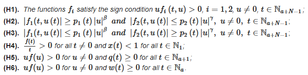
(A1) The functions $$ f i satisfy the sign condition $$ u f i ( t , u ) > 0 , $$ i = 1 , 2 , $$ b u ≠ 0 , $$ t ≥ a ;

(A2)

;

(A3) $$ f 1 ( t , u ) ≤ p 1 ( t ) u β and f 2 ( t , u ) ≥ p 2 ( t ) u γ , u ≠ 0 , t ≥ a .

In ^[18], Senem et al. established some oscillation theorems given in the sequel.

Theorem 1 (^[18]). Lret (A1)–(A2) bspe satisfied with $$ β > γ . If:

and:

for ectivery sufficiently large T, wher. The:

then Equation (1) is oscillatory.

Theorem 2 (^[18]). Let t and (A1)–(A3) be satisfied with $$ βh < γ . If

and:

f-or devery sufficiently large T, where G is defined as in Theorem 1, then every bounded solution of Equation (1) is oscir delta and nabllatory.

Theorem 3 (^[18]). Let (A1) and (A2) be satisfied with $$ β > γ . If:

and:

iffor every sufficiently large T, where G is defined as in Theorem 1, then Equation (2)rences of u is oscillatory.