Your browser does not fully support modern features. Please upgrade for a smoother experience.
Please note this is a comparison between Version 2 by Jnanada Shrikant Joshi and Version 1 by Andrea Ehrmann.
Atomic force microscopy (AFM) is one of the microscopic techniques with the highest lateral resolution. It can usually be applied in air or even in liquids, enabling the investigation of a broader range of samples than scanning electron microscopy (SEM), which is mostly performed in vacuum. Since it works by following the sample surface based on the force between the scanning tip and the sample, interactions have to be taken into account, making the AFM of irregular samples complicated, but on the other hand it allows measurements of more physical parameters than pure topography.
- nanoindentation
- elastic modulus
- peak force quantitative nanomechanical mapping
- KPFM
1. Introduction
The topography, roughness and similar morphological parameters of surfaces are often investigated by microscopic methods. These parameters are not only important in materials sciences, during the development of new materials with different surface morphologies, but also in biotechnology and many other research areas where a substrate’s surface plays an important role for the adhesion of other materials or living cells, etc.
While light microscopy has been well-known for hundreds of years [1], electron microscopy has not even been used for a century now [2], and AFM was first mentioned only in 1986 [3]. Since then, it has rapidly had more and more impact in microscopy techniques, as depicted by Parot et al. in their review of the history of AFM in the life sciences [4]. In 1987, the first measurements in liquid were performed, the first membrane proteins were depicted in 1991, in 1997 the first single protein unfolding was observed, and in 2004, the native organization of membrane protein supercomplexes were reported, etc. From year to year, technical innovations have been added, such as new cantilevers, the tapping mode often used on biological samples, high-speed techniques, and many more [4], leading to the recent state in which many biological and biotechnological research groups use an AFM as naturally as a fluorescence microscope. The main advantage of an AFM against light microscopes is its resolution which may reach that of single atoms on a flat sample surface for inorganic matter, while the AFM of functional biomolecules in aqueous solutions has been shown to achieve a resolution around 1 nm, which is identical to the smallest tip radius [5]. For a less powerful resolution, AFM images can be taken in the air or in liquids, making it also advantageous for biological—usually water-containing—tissue in comparison to scanning electron microscopy (SEM) which mostly needs a vacuum in the sample chamber [6].
2. AFM Techniques
The atomic force microscope is recently the most often used scanning probe microscope. Its general working principle can be described as follows: a tip, often produced from Si or Si3N4 and with a typical tip radius around 1 nm to 20 nm, sometimes larger, is attached to the end of a cantilever. The cantilever can vibrate with a specific spring constant, typically with frequencies around some ten to a few hundred kilohertz. By measuring the signal on a photodiode, the z-position of the cantilever holder is usually moved so that a constant force between the tip and the surface is maintained. This moving z-position is transferred into the surface topography. The forces between the tip and the surface are mostly—without an additional functionalization of the tip—based on electrostatic Coulomb forces (repulsive) and van der Waals forces (attractive) and are exceedingly small, approx. in the range of 10−11 N to 10−7 N. The distinctly small distances between the tip and surfaces—typically around 0.1 nm to 10 nm—enable a resolution in the order of 0.1 nm under perfect conditions, especially in the case of a perfectly smooth surface. Other forces, however, may superpose the aforementioned ones and have to be taken into account during the interpretation of AFM images [7].2.1. Topography and Roughness
The cantilever can approach the sample surface in different ways—either in the contact mode [8]. While the resolution can be higher in the contact mode, the lateral forces due to the friction between the tip and sample may be problematic for soft or uneven surfaces, which is why for such samples often the dynamic mode is chosen. This means that the cantilever performs oscillations near its resonance frequency and only taps towards the sample briefly, so that the lateral movement can be performed without the tip sticking to the sample surface [8]. It should be mentioned that in the so-called noncontact mode, the cantilever also vibrates, but with a smaller amplitude, thus not touching the sample surface. Yang et al. reported that the noncontact mode exerts a delicate force on the sample at the cost of less precise height measurements, while the tapping mode caused deformations of the soft materials, especially in liquid environments [9]. Such topography investigations have been performed on many different materials during the last decades, e.g., on food biopolymers [10], on biopolymer networks [11], proteins and DNA [12,13], or hydrogels [14].
Topography measurements also allow calculating the surface roughness, which is especially interesting for homogeneous, isotropic surfaces, while anisotropic morphologies—e.g., from nanofibers or fibroblasts—usually give more information in the full topography image.
By measuring the cantilever deflection, which is correlated to the force on the tip, during vertical displacement, it is also possible to measure force-distant curves in the so-called force spectroscopy mode, which allows for detecting interaction forces between the tip and sample as well as an elastic modulus (Young’s modulus) which may vary from the values from macroscopic tests, but is actually supportive for the evaluation of microorganisms, nanoparticles, hydrogels or other small-scale samples [8]. The force-distance curve shows an increasing force during approaching (red part of the curve), based on electrostatic and van der Waals forces. During retraction, firstly the tip sticks to the surface due to adhesive forces, leading to a strong decrease in force, i.e., a negative cantilever deflection, before it becomes free and the force approaches the original one again.
Generally, such forces are quite small for cells, tissue, soft hydrogels and biopolymers in different forms. It should be mentioned that by functionalizing the AFM tip with specific groups or molecules, even more information can be gained from the interaction between the sample and the functionalized tip [16].
2.2. Phase Imaging
Phase imaging belongs to the standard modes of an AFM and is thus usually also recorded when topography images are taken in the tapping mode. The corresponding images show the phase between the piezo-driven excitation and the actual oscillation of the cantilever. Since this phase depends on the sample hardness, elasticity and adhesion, it allows for distinguishing different materials in a sample; however, only in a qualitative way [17].
Moreover, the phase image increases the visibility of edges, sometimes making small features more visible [7]. This is especially interesting for highly irregular surfaces, where the feature height necessitates relatively large free vibration amplitudes of the cantilever which lead to a lower noise level, but also lower the resolution. As an example, from our own research, Figure 1 shows AFM measurements under identical conditions on two poly(acrylonitrile) (PAN) nanofiber mats after electrospinning (Figure 1a) and after hot-pressing at 180 °C (Figure 1b). These topography maps show that after hot-pressing, the fibers become thicker, as expected. In Figure 1a, however, the fibers look more like high walls, which is not possible. This artifact is not visible in the phase image of the raw nanofiber mat (Figure 1c), where the areas between the clearly separated fiber surfaces show different phases. This finding can be attributed to small movements of the nanofibers during scanning, making them look broader in the topography image. On the other hand, Figure 1d clearly shows dark lines in the phase map of the hot-pressed sample. These lines are not related to the aforementioned material variations, as they are also slightly visible in the topography (Figure 1b), but they show topographical constrictions upon heating, as they are also known from the thermal stabilization of PAN nanofiber mats [18,19].
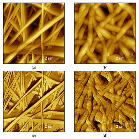
Figure 1. AFM images taken on poly(acrylonitrile) (PAN) nanofiber mats: (a) raw mat, topography image; (b) hot-pressed mat, topography image; (c) raw mat, phase image; and (d) hot-pressed mat, phase image. Images taken with a Nanosurf FlexAFM with the following scanning parameters: 512 points × 512 lines, 1.4 s/line, setpoint 55%, p-gain 550, i-gain 1000, d-gain 100, free vibration amplitude 6 V.
Besides this relatively simple technique, many more modes can be applied with most modern AFM instruments, partly with modified equipment and often applying specialized cantilevers, partly by simply changing the measurement parameters. On the other hand, small changes in the measurement situation can have a large impact on the results, as the next section shows.
2.3. Attractive and Repulsive Interaction Regimes
In the tapping mode, the cantilever oscillated near its resonance frequency, and the amplitude reduction due to the forces between tip and surface is measured. This amplitude modulation feedback is influenced by attractive as well as by repulsive forces. This means, on the one hand, that a distance where parts of the sample show repulsive forces of similar dimension as the attractive forces in other sample parts will lead to a low contrast as no differentiation between both is possible [20]. García and San Paulo calculated the discontinuities in the amplitude and phase shift curves for crossing the border between both regimes [21] and described different possibilities for how the amplitude could be related to the displacement between the tip and sample, measured on different samples with varying free amplitudes [22]. In some cases, the amplitude is insensitive to displacements for larger distances than approx. 15 nm, while a linear correlation is found for smaller distances. In both other cases, however, there is a local maximum which they attribute to the competition of different interaction regimes, i.e., long-range attractive and short-range repulsive forces, causing possible problems in the interpretation of the corresponding topography images.
The differentiation between two interaction regimes, however, can not only cause problems, but also be used to choose the optimum regime for a specific measurement. Round and Miles, e.g., report a contrast change in topography and phase images during measurements on DNA in air, which they attributed to a nonlinear dynamic response of the cantilever near the surface, i.e., near a repulsive barrier [23]. They showed that by slightly modifying the driving frequency around the resonance frequency, the topography and phase contrast could be varied and even switched off. San Paulo and García mentioned that in the repulsive regime, usually the contrast and resolution were reduced, combined with damaging the tip due to the forces between the tip and the sample [24].
An interesting point was raised by Zitzler et al. who investigated the influence of relative humidity on measurements on hydrophilic samples [25]. They showed that generally an adsorbed water layer on the sample surface could interact with the tip due to capillary forces. When the cantilever oscillates with sufficiently high amplitude near the sample surface, a capillary neck could be formed between the tip and the sample, leading to a hysteresis in the force-distance curve which may especially be important for samples with locally varying wettability, as often found in biological samples. This effect was also shown for contact-mode measurements [26,27].
Maragliano et al. used the transition between attractive and repulsive force regimes for the evaluation of the tip radius [28]. They showed that for a sharper tip, the value of the free amplitude leading to a transition between these regimes was smaller. On the other hand, they used capacitance-distance curves combined with an analytical model. The first method, measuring the minimum critical amplitude to reach the border between both regimes, i.e., bistable behavior, was found to give more accurate results especially for fine tips.
2.4. Nanoindentation
Nanoindentation in the AFM can be used to evaluate the mechanical characteristics of biological and other samples. Such experiments are performed by indenting the AFM tip into the sample and retracting it again, leading to load-indentation curves, as shown in Figure 2 [29]. The authors describe different possibilities for the evaluation of such experiments, i.e., the most often used Hertz model and the Oliver and Pharr analysis, and evaluate the influence of the indenter shape. They found clear differences for not perfectly elastic samples and suggested the Hertz model only in this case. Recently, Kontomaris et al. discussed an extension of the Hertz model for biological samples including indentation depth, tip radius, and sample shape to overcome problems with the common Hertz model [30].
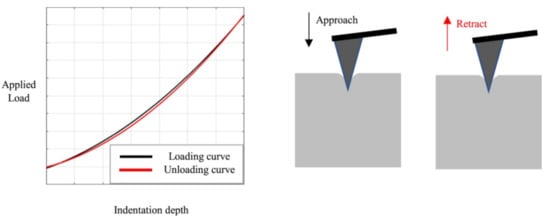
Figure 2. Indentation experiment with loading and unloading curves. Reprinted from [29], originally published under a CC-BY license.
Qian and Zhao reviewed nanoindentation especially for soft biological materials [31]. They mentioned that for soft biological samples, relatively soft tips could be used, such as silica or silicon, aluminum or steel in addition to the typical materials for nanoindentation such as sapphire or diamond. Similarly, they found large tips in the range of millimeters being used for particularly soft biomaterials and suggested using a tip size much smaller than the tissue and much larger than an individual cell or fiber in the case of tissue-level experiments. Similar materials and dimensions as well as different tip shapes were mentioned by Vlassov et al., reviewing nanoindentation experiments on polydimethylsiloxane (PDMS), a silicon-based organic polymer often used in microfluidics and other areas [32].
Sokolov et al. mention for the special case of nanoindentation on eukaryotic and Gram-negative prokaryotic cells that the brush surrounding them has to be taken into account, and that these experiments enabled measuring the length and grafting density of the brush [33]. They formulated some rules regarding nanoindentation on cells, such as working only on the flat part of a cell, keeping the vertical ramping speed constant, checking the linearity of the mechanical response of the cell body material, and collecting enough data per cell for a proper statistical treatment.
Finally, Guo and Roos showed that nanoindentation on protein shells was even possible in liquids, i.e., similar to the physiological environment [34].
2.5. Peak Force Quantitative Nanomechanical Mapping (PeakForce QNM)
Another method to determine the elastic modulus of a sample is the PeakForce QNM technique. The PeakForce QNM tapping mode works similar to the normal tapping mode, with the difference that in the common tapping mode the cantilever vibration amplitude is kept constant, while in the peak force mode the maximum force is controlled to avoid damage of the tip or sample [35]. They described measuring the architecture of an intact plant cell in fluid by this technique.
Dokukin and Sokolov compared PeakForce QNM measurements on polyurethanes and polystyrene with results from nanoindentation and other techniques and found that, for sharp probes, the PeakForce QNM measurements overestimated the elastic modulus, while dull AFM probes with tip diameters around 240 nm could be used for quantitative mapping of the elastic modulus with a resolution of approx. 50 nm [36].
Zhou et al. used the PeakForce QNM to investigate bovine cortical bones in water [37]. They found differences in the elastic moduli of osteons, interstitial bones, cement lines and different sub-lamellae and could visualize soft mineralized collagen fibrils in a harder matrix. The elastic moduli were measured and modeled, based on the Derjaguin–Muller–Toporov (DMT) model with a Hertzian contact profile which was used to fit the load-deformation curves for the tip retraction process. DMT modeling was also used by Schön et al. for mapping the elastic moduli in phase-separated polyurethanes [38]. Generally, for systems with low adhesion and small tip radii, the DMT theory is advantageous, while the Johnson–Kendall–Roberts (JKR) theory is used for highly adhesive systems with low stiffness and large tip radii, and the Hertz theory is only suitable for negligible adhesion forces [36].
2.6. Hardness Measurements
Hardness measurements on different samples can be performed, similar to elasticity measurements, by nanoindentation. Here again, the indenter shape and the tip radius have to be taken into account during the interpretation of the measured curves. Calabri et al. calculated correction factors for different tip curvature radii [39]. They mentioned that the tip radius is less important for the indentation process itself, but for the subsequent imaging process of the area impressed during indentation. These findings could also be used to model the effect of worn tips on nanoindentation correctly. With these corrections, hardness measurements by AFM only slightly underestimated the hardness in comparison with typical literature values.
While some groups investigated the special challenges related to thin-film systems and rough surfaces, e.g., by reducing the necessary indentation depth [40], for biomaterials it is often more important that working under water is possible. This was shown, e.g., by Balooch et al. who compared hardness and elastic modulus measurements of demineralized human dentin in water, in air after desiccation and in water after rehydration [41]. They found strong differences between the viscoelastic values and elastic moduli measured in water and after desiccation, while rehydration did not fully bring the original values back, which was attributed to oxidation-induced crosslinking and chain entanglement of the collagen upon drying. It must be mentioned that the fully hydrated dentin specimens did not have a measurable hardness value since it was impossible to reach a permanent deformation by nanoindentation.
2.7. Adhesion Measurements
For adhesion measurements, many authors report on using cantilevers with an increased adhesion area, e.g., by using an elastomeric colloidal probe [42]. Erath et al. applied the aforementioned Johnson–Kendall–Roberts (JKR) approach, measuring the contact area as a function of load combined with elastic parameters, to distinguish between the capillary forces in air, hydration forces and hydrophobic interactions in water for the interaction between the soft colloid and the substrate.
Dong et al. investigated the adhesion between a protein and a TiO2 substrate by using a lysozyme-modified tip [43]. The adhesion was measured by the force jump upon retraction, i.e., identified as the pull-off force necessary for separation of the tip from the surface. Similarly, Wojcikiewicz et al. attached 3A9 cells by concanavalin A-mediated linkages to an AFM cantilever, approached the sample until the cell was in contact with the surface, and retracted the cantilever with the cell until separation, in this way measuring the detachment force [44]. The adhesion between the DNA and living cells was measured in a similar way by Hsiao et al. using DNA-coated cantilevers and measuring the de-adhesion force during retraction of the cantilever [45].
Besides the topological and mechanical properties described in the previous sections, it is also possible to measure the chemical or electronic properties of specimens. Some of the techniques related to biopolymers and hydrogels are described in the next sections.
2.8. Kelvin Probe Force Microscopy
Kelvin probe force microscopy (KPFM) allows for mapping the surface potential of a sample [46]. This electrical AFM mode measures the difference in work function or contact potential difference between the tip and the sample surface [47]. The work function defines the minimum energy necessary for an electron to leave the surface of a material. While the work function is often mentioned in correlation with metals, biomolecules also have a work function, i.e., an energy difference between the “outer” electron in the sample and the vacuum level [48]. It is influenced by local electromagnetic and also mechanical properties, such as surface charges, dielectric constants or the doping level of a semiconductor.
Generally, KPFM is measured with conductive probes whose work function can be calibrated on highly-oriented pyrolytic graphite (HOPG) for which the work function in air is well-known. When the AFM tip is near the sample surface, an electrical force occurs due to the difference in Fermi levels [49]. Leveling out this additional electrical force by an external bias voltage (combining an AC and a DC signal) enables calculating the contact potential difference and thus the material’s work function. It is still necessary to distinguish between the electrical and topography signal, which can be completed with a high-frequency AC voltage combined with a sophisticated evaluation, depending on the measurement mode (frequency modulation or amplitude modulation measurement).
While some groups work on measuring and interpreting highly resolved KPFM images on the atomic scale [50], for biomaterials the KPFM measurements in liquid are more interesting, which are indeed possible, as described by Collins et al. [51].
2.9. Conductive AFM
Another electric measurement type is conductive AFM or conducting probe AFM, also called C-AFM or CP-AFM. It can be used, e.g., to measure the varying thickness of an oxide film on a semiconducting substrate [52] or the resistance of semiconducting nanowires [53].
Molecular crystals from sexithiophene were investigated by CP-AFM, using Au-coated Si probes to reduce the contact resistance [54]. They found resistances of a few hundred MΩ along some hundred nanometers, with significantly higher resistances around a few hundred GΩ if the measurement was performed via a grain boundary. Other typical probes are Si with a Pt/Ir coating [55] or with a chromium buffer layer followed by gold [56]. For measurements on molecular wires by CP-AFM, Ishida et al. reported apparently negative differential resistance values at a higher bias which they attributed to the surface roughness, and a strong influence of the tip-molecule contact on the carrier transport through the system [57].
Concluding, Table 1 gives a brief overview of the similarities and differences of the AFM modes mentioned in this section.
Table 1. Characteristics of different AFM modes.
| AFM Mode | Information Given | Static/Dynamic Mode | Special Requirements |
|---|---|---|---|
| Contact mode | Topography, roughness | Static mode | Cantilever for static mode |
| Tapping mode | Topography, roughness | Dynamic mode | Cantilever for dynamic mode |
| Phase imaging | Qualitative differentiation between materials + clearer edges within single material | Dynamic mode | Cantilever for dynamic mode |
| Nanoindentation | Elastic modulus, hardness | Dynamic/static/quasistatic | Tip harder than sample |
| PeakForce QNM | Elastic modulus, adhesion | Dynamic mode | Often very broad tips are supportive, functionalization of the cantilever broadens the measurement spectrum |
| KPFM | Contact potential (work function) of a surface | Dynamic mode | Conductive tip, single or dual pass setup |
| Conductive AFM | Conductivity; local current-voltage curves | Static mode | Conductive tip |