Your browser does not fully support modern features. Please upgrade for a smoother experience.
Please note this is a comparison between Version 2 by Conner Chen and Version 1 by Olesja Starkova.
Substantial gains and savings of resources of time and money can be gained through the use of modelling and simulation to understand material system performance. Since for development of the new materials validation is expensive and time-consuming, the bottleneck is time and funding—modelling might be the way to replace testing programs, which would be beneficial for providing new innovative materials faster to the market.
- modelling
- lifetime prediction
- accelerated testing methods
- durability
- mechanical properties
- creep
- fatigue
1. Arrhenius Model
1. Rate Models
1.1. Arrhenius Model
The Arrhenius model is widely used when temperature is the dominant accelerating factor in ageing. It is assumed that a single dominant degradation mechanism does not change during the exposure period, while the degradation rate is accelerated with an increase of exposure temperature [14]. The Arrhenius relation is given by
where K is a reaction rate or degradation rate, A is a constant related to material and degradation process, Ea is the process activation energy, R is the universal gas constant, and T is the absolute temperature. The degradation rate is proportional to the inverse time for degradation of a mechanical property for a given value set by the lifetime criterion, and log(t) vs. 1/T is a linear function with the slope Ea/R (Figure 21). The Arrhenius relationship is widely used for lifetime predictions of polymers and composites through monitoring ultimate mechanical properties and their retention, e.g., tensile strength, interfacial shear strength, creep strength, and fatigue strength [6,21].
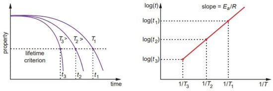
Figure 21.
Lifetime prediction according to the Arrhenius model.
The durability prediction methodology in most studies is based on the time shift concept [8,21,22,23,24,25,26,27]. According to Equation (1), the time shift factor (TSF) for two different exposure temperatures T1 and (T1 < T2) can be calculated as
Equation (2) has been further used in the predictive methods based on superposition principles and assessment of the temperature shift factors (Section 2.2). The activation energy in Equations (1) and (2) is commonly evaluated by thermal analysis methods, e.g., differential scanning calorimetry or thermogravimetric analysis by measuring heat capacity changes or mass losses under different heating rates. Alternatively, Ea can be determined by dynamic thermal mechanical analysis (DMTA) assessing Tg dependence on the test frequency [28,29].
Some recent studies considering the Arrhenius model and TSF approach for predicting the long-term strength of various FRP are listed in Table 1. Note that this methodology can be applied for assessment of tensile strength [22,30], interlaminar shear strength [23,26,27] or bond strength [25], under both static and fatigue loadings [26]. The accelerating temperature effect can also be coupled with other factors, e.g., absorbed water. For instance, Gagani et al. [26] applied the time shift concept to assess interlaminar shear fatigue lifetime of GFRP considering the effects of temperature and water immersion. The glass transition temperature of the material, and its decrease due to absorbed water, was used in Equation (2), enabling representation of both dry and water saturated samples in the same Arrhenius-based master curve.
Table 1. A condensed list of recent works on methods for predicting long-term mechanical properties of polymers and polymer composites.
| Prediction Method | Material | Property | Ref. |
|---|---|---|---|
| Rate models | |||
| Arrhenius model | GFRP | Tensile strength | [22,30] |
| GFRP | ILSS | [27] | |
| GFRP | Fatigue ILSS | [26] | |
| GFRP bars | Tensile strength | [8] | |
| CFRP/GFRP rods | ILSS | [23] | |
| BFRP bars | Residual tensile strength | [24] | |
| GFRP rods | Bond strength | [25] | |
| Eyring’s model | PA6,6, PC, CFRP | Creep failure time | [31] |
| Zhurkov’ model | PP | Fatigue strength | [32] |
| Superposition principles | |||
| Time–temperature (TTSP) | Epoxy | Creep compliance | [28,33] |
| Epoxy | Stress relaxation | [34] | |
| Filled epoxy | Stiffness/Relaxation modulus | [35] | |
| PMMA | Creep compliance | [36] | |
| Polyvinyl chloride, epoxy | Stress threshold of LVE | [37,38] | |
| Flax/vinylester | Creep compliance | [39] | |
| CFRP | Creep compliance | [40,41] | |
| CFRP, GFRP | Static/creep/fatigue strength | [42,43] | |
| Time–moisture (TMSP) | Epoxy | Creep compliance | [28,33] |
| Epoxy | Relaxation/storage modulus | [44,45,46,47,48] | |
| Epoxy-based compounds | Relaxation modulus | [49] | |
| Vinylester | Creep strain | [50] | |
| Polyester | Creep strain | [51] | |
| PA6, PA6,6 | Storage modulus | [47,52] | |
| CFRP, GFRP | Fatigue strength | [53] | |
| Time–stress (TSSP) | PA6 | Creep strain | [54] |
| PMMA | Creep compliance | [36,55,56] | |
| HDPE | Creep strain/lifetime | [57] | |
| Polycarbonate | Creep compliance | [58] | |
| PA6,6 fibres | Creep strain | [59] | |
| Glass/PA, PP, HDPE | Creep compliance | [60] | |
| HDPE/wood flour | Creep strain | [61] | |
| Graphite/epoxy FRP | Creep strain | [62] | |
| Kevlar yarns, PA6, epoxy | Creep strain (stepped isostress test) | [63,64,65] | |
| Coupled | |||
| TTSP + TMSP | Epoxy | Creep compliance | [28] |
| TTSP + TMSP | PA6,6 | Storage modulus | [52] |
| TTSP + TMSP | Acrylate-based polymers | Storage modulus | [66] |
| TTSP + TMSP | CFRP, GFRP | Static/creep/fatigue strength | [53,67] |
| TTSP + TSSP | HDPE/wood flour | Creep strain | [61] |
| TASP+TMSP | Epoxy, polyester | Creep compliance, stress relaxation | [44,45] |
| TTSP+TASP | Epoxy | Relaxation modulus | [34,68] |
| TTSP+TASP+TSSP | PMMA | Creep strain | [55] |
| Plasticity-controlled failure | PP, PP/CNT, glass/PP, carbon/PEEK, PC/GF, PA6 | Lifetime (tensile, creep, fatigue) | [69,70,71,72,73,74] |
| PA6,6, PC, CFRP | Creep lifetime | [31] | |
| Parametric methods | HDPE | Creep lifetime (Larson–Miller, Monkman–Grant) | [57] |
| GFRP | Creep lifetime (Monkman–Grant) | [75] | |
| Rubber-bonded composite | Creep lifetime (Larson–Miller) | [76] | |
| Adhesive anchor in concrete | Creep lifetime (Monkman–Grant) | [77] | |
| Short fibre thermoplastics | Fatigue lifetime (Larson–Miller) | [78,79] |
1.2. Eyring’s Model
2. Eyring’s Model
The reaction rate of a process can rely on several stressors. For example, nonthermal stresses such as humidity, voltage and mechanical stress may also play a significant role in accelerating degradation [14]. The Eyring model is based on chemical reaction-rate theory and describes how the rate of degradation of a material varies with stress. It is assumed that the contribution of each stressor to the reaction rate is independent; thus, one could multiply the respective stress contributions to the rate of reaction. The model is closely related to the Arrhenius model and is based on the fact that the logarithm of the reaction rate is inversely proportional to absolute temperature (Equation (1)).
According to Eyring’s thermal activation flow theory, the strain rate (or the characteristic time) is given by the relationship
ε˙=1t=A1exp(−Ea−γσRT)
1.3. Zhurkov’s Model
3. Zhurkov’s Model
Zhurkov developed the kinetic theory of strength of solids using temperature and tensile stress [32,81]. The relationship for calculation of the fracture lifetime tf is similar to Equation (3), while the coefficient γ referred to as the lethargy coefficient is linked to lattice structure and defects in it. In the general case of nonisothermal tests and σ varying in time (e.g., creep and fatigue tests), the fracture probability with account of the linear damage accumulation concept is given by the following equation [32,75,82]:
where t0 is the time constant.
∫0tfdtt0exp(Ea−γ(σ(t))RT(t))=1
Zhurkov’s model initially developed for metals often could not give accurate lifetime predictions for polymers owing to the sensitiveness of their mechanical properties to strain rate and uncertain distinctions between the elastic and plastic ranges. As a result, the parameters involved in Equation (4) are interrelated stress, temperature, and strain-rate dependent functions. The kinetic concept of strength is applied to model fatigue damage evolution [32,83]. Hur et al. developed a modified Zhurkov’s fatigue life model introducing strain-rate-dependent lethargy coefficient and applied it to polypropylene reinforced with glass fibres [32]. The stress-based failure cycles in the ranges of low- and high-cycle fatigue were predicted and successfully validated by the proposed modified strain-rate model. The kinetic strength model applied to lifetime predictions of biodegradable polymers is discussed in the review paper by Laycock et al. [5]. For this type of material, Zhurkov’s equation is coupled with broader biodegradation models enabling assessment of stress effects on the lifetime via lowering the activation energy for chain scission.
2. Superposition Principles
Environmental ageing affects relaxation properties of polymers manifest in accelerated viscoelastic response (e.g., creep compliance, relaxation modulus) and time-dependent failure. This fact is widely applied to predict the long-term properties of polymer composites by using superposition principles and extending the time span. Depending on the accelerated factor, different methods are used: time–temperature superposition principles (TTSP), time–moisture superposition principles (TMSP), and time–stress superposition principles (TSSP). In other superposition principles, changes in the viscoelastic response are related to an ageing mechanism rather than a factor itself, e.g., time–physical ageing or time–curing degree [34,44,45,55,68], time–plasticization [28], time–hydrothermal ageing [46], and other superposition principles. Literature data on different superposition principles applied to various polymers and composites are summarised in Table 1.
Superposition principles are based on the assumption that time t and a factor f, which accelerates the relaxation processes (e.g., temperature T, moisture content w, and stress σ) are interrelated and interequivalent. The action of factor f leads to a parallel shift of the relaxation spectrum τi for a value af. For the reduced or effective time, this can be written as follows: τ′i=τi/af or
where af is the shift factor and f could be T, w, σ, or other. The concept of effective time allows one to correlate two time scales: the intrinsic time scale of the material revealed by viscoelastic relaxation and the observation time measured directly by a watch. Thus, it is possible to extend the observation time by influencing the intrinsic time by an external factor.
t′=taf
In a general case, the accelerating factor could change during the loading history, then the shift factor Equation (5) transforms into a time-dependent function as
t′=∫0taf[f(s)]ds
Under simultaneous action of several accelerated factors, e.g., f1 and f2, the total shift factor is contributed by both constituents:
af1,2=F(af1,af2)
Under additive contribution of environmental factors, i.e., when their action could be regarded separately, the time scale shift is realised by using a simple product of single shift factors, i.e., af1,2=af1×af2.
2.1. Time–Temperature Superposition Principle
TTSP is one the most widely used prediction methods mainly due to its technical simplicity, controllability of testing procedures, and tractability of the obtained results. The schematic of long-term prediction of creep compliance by TTSP is shown in Figure 3. The viscoelastic property, e.g., creep compliances, at two different temperatures T0 and T1, differ only by a time scale defined by the temperature shift functions aT0 and aT1. Creep compliances J can reach the same values at different time moments t0 and t1, i.e., J(t0,T0)=J(t1,T1) or according to Equation (5) t0aT0= t1aT1 and logt0−logt1=logaT1− logaT0. For simplicity, the reference shift factor is typically taken as unity aT0=1. Thus, the creep compliance curves in logarithmic time axes are parallel for different T and shifted to each other for values logaT. The long-term prediction is represented by the generalised master curve (Figure 3). The concept of time-shift factors allows one to estimate the ratio between times required for a certain decrease in a mechanical property at two different operating temperatures [8,22]. Similar considerations are valid for other accelerated factors and related superposition principles. Applicability of TTSP has also been a validated methodology to determine the energy limit and stress threshold of linear viscoelastic behaviour of various polymers [37,38,84].
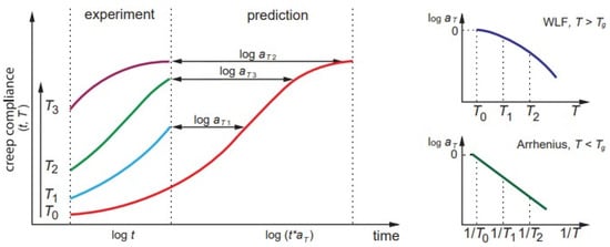
Figure 3. Superposition principles by the example of TTSP for creep compliance.
It should be noted that the procedure described is valid for thermorheologically simple materials exhibiting linear viscoelastic behaviour. However, it could be used in more complex cases after some modifications, e.g., vertical shift functions [57,85], stress-dependent parameters [35], equivalent strain rate [52], etc. The vertical shift factors could result from changes in the structure, e.g., degree of crystallinity in semicrystalline polymers [86] or residual curing in thermoset resins [39,87]. They can also be associated with the stress-dependent effects of nonlinear viscoelasticity [36]. Time–temperature shift factors are affected by the physical ageing of a material. As a result, superposition will not work if the testing time is comparable to the ageing time of the material. According to Barbero [88], experiments for TTSP should be performed on a timescale at least ten times shorter than the ageing time of the sample (see also Section 2.2.4).
The mathematical relationships for the temperature shift functions depend on the temperature range considered. The Williams–Landel–Ferry (WLF) equation is valid for T between Tg and Tg +100 °C [89]:
where C1 and C2 are material parameters.
logaT=−C1(T−T0)C2+T−T0
The Arrhenius equation is applied for aT calculations of glassy polymers at T < Tg [89]:
where the temperature is taken in Kelvin and other symbols are the same as in Equation (1).
logaT=−Ea2.303R(1T−1T0)
Equation (9) is sometimes used for aT calculations above Tg, although with a different Ea value, i.e., slope in logaT vs. 1/T line (Figure 3). A generalised relationship for the time–temperature shift factor valid in a full operating temperature range is defined as follows [85,90]:
where H is the Heaviside step function; Ea1 and Ea2 represent the activation energies below and above Tg, respectively.
logaT=Ea12.303R(1T−1T0)H(Tg−T)+[Ea12.303R(1Tg−1T0)+Ea22.303R(1T−1Tg)]×(1−H(Tg−T))
As far as the shift factors are known, the lifetime of a polymer system t at an operating temperature T can be determined according to Equation (5) by the ratio [6]:
where t0(T0) is the lifetime at the reference temperature.
t(T)=aT0aT⋅t0(T0)
In the case of FRP, the temperature effect is associated with the viscoelastic properties of the polymer matrix [40,41]. Thus, the temperature shift factors usually are the same for the polymer and composite. This fact is employed in the accelerated testing methodology for the long-term durability of various FRP [42,43] (see also Section 2.5.2).
2.2. Time–Moisture Superposition Principle
In TMSP, absorbed moisture (water) is considered a factor that accelerates the relaxation processes. The analogy between plasticizing effects of temperature and moisture on the viscoelastic behaviour of polymers is mentioned in several pioneering works: Onogi et al. [91], Maksimov et al. [92], Flaggs and Crossman [93], and Weitsman [94].
The general procedure for long-term prediction is similar to that in TTSP: short-term data are obtained at a fixed temperature for samples with different equilibrium water contents. The master curve is constructed by horizontally shifting these data to a reference curve (typically, a dry sample). An example of TMSP applied to long-term creep of vinylester resin is shown in Figure 4 [50].
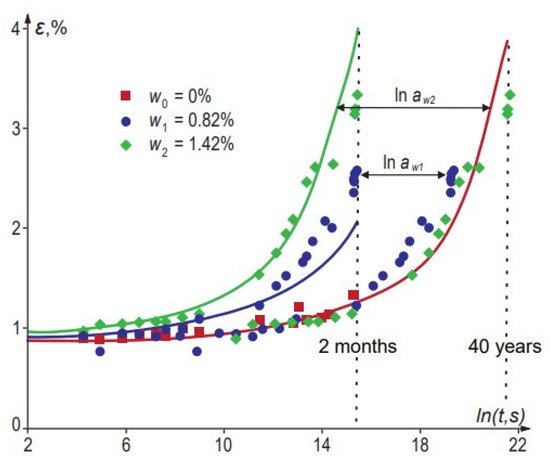
Figure 4. Creep curves of vinylester with different equilibrium moisture contents (w0, w1, w2) and the master curve constructed by applying TMSP. The Boltzmann–Volterra equation calculates the line for the linear viscoelastic solid and time–moisture shift function given by Equation (13). Data are taken from [50].
The time–water content shift factor aw can be expressed by the relationship similar to the WLF equation (Equation (8)) [47,52]:
where w and w0 are water contents in the “wet” and reference states, respectively. D1 and D2 are material constants determined from experimental data; logaw can also be given by a polynomial [44,50,51,95]:
where d1 and d2 are empirical coefficients.
logaw=−D1(w−w0)D2+w−w0
logaw=d1(w−w0)+d2(w−w0)2
The plasticizing effect of absorbed water is manifest as a Tg drop. The Fox model [52,53], also known as Simha–Boyer model [96], is among the most known models used for the prediction of Tg variations with w:
where Tg0 and TH2Og (−150 °C) are Tg of the “dry” polymer and water, respectively. Tg drop per 1% of absorbed water usually is in the range of 5–10 °C for epoxy systems [28,29,47,96] and 20–40 °C for polyamides [47,52].
1Tg=(1−w)Tg0+wTH2Og
Considering Tg as an indicator of polymer chain mobility related to its free volume, Krauklis et al. developed the time–temperature-plasticization superposition principle [28]. The moisture (called plasticization) shift factors were determined by the Arrhenius-type equation (Equation (9)), changing operating temperatures to Tg of the dry and plasticized (Tgw) polymer [28]:
logaw=−Ea2.303R(1Tgw−1Tg0)
An application on amine-cured epoxy validated the proposed method; this particular epoxy material system and the underlying mechanism of ageing are described in more detail in [97,98,99]. The activation energy Ea, determined by DMTA and assessment of Tg changes with the test frequency, was found to be the same for dry and moisture-plasticized polymer. The moisture shift factors logaw calculated by Equation (15) correlated well with those determined by a common shifting of the creep compliance curves [28].
By combining Equations (14) and (15), it is possible to calculate logaw for material with any moisture content. The only parameters involved are Tg0 and Ea that could be determined by thermomechanical methods without performing time-consuming creep tests. Then, according to Equations (11), (14), and (15), the lifetime of a plasticized polymer can directly be assessed from Tg changes.
TMSP has been applied for various polymers and polymer composites, and a list of some works is given in Table 1. The great majority of them are related to different epoxy systems [28,33,44,45,46,47,48,49] and epoxy-based composites [49,53], along with some other polymers, e.g., polyester [51], vinylester [50], and polyamide [47,52]. TMSP is often coupled with other superposition principles, e.g., TTSP, when studying temperature effects on dry and wet materials [28,52,53,66,67,100]. Some other rheological models that consider water plasticization effects on viscoelastic–viscoplastic behaviour epoxy and epoxy-based composites are discussed in [101,102]. Xiao and Li studied plasticizing effect of solvents on viscoelastic properties of gels and applied TTSP with the shift factor described by the WLF equation [103].
2.3. Time–Stress Superposition Principle
The time–stress superposition principles (TSSP) allow accelerated testing of materials to determine their creep response and creep-rupture behaviour. The testing procedure is similar to that in TTSP (Figure 3), but the acceleration is obtained by increasing the stress instead of temperature. An example of TSSP applied to creep of PA6,6 fibres is shown in Figure 5: data of short-term tests are shifted to the master curve that gives the creep prediction for extremely long times [59]. TSSP is advantageous compared to TTSP because there is no need to use elevated temperatures, which may alter the chemical structure of the polymers tested. This fact is used in the related prediction technique, i.e., the stepped isostress method (SSM), allowing construction of the entire creep master curve by testing only one sample subjected to successively increasing stepped stresses [62,63,64,65]. At the same time, TSSP could have some limitations in terms of stress and time due to the differences in creep mechanisms under low and high loads.
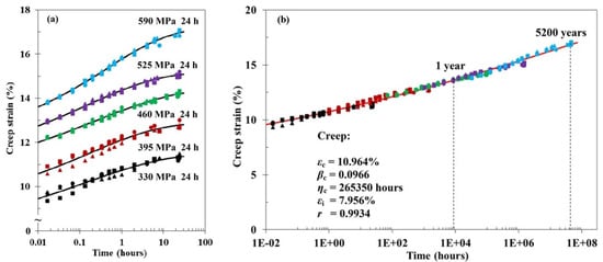
Figure 5. Creep curves for PA6,6 fibres at various creep stresses (a) and master curve obtained by TSSP (b). Adopted with permission from Ref. [59]. Copyright 2017 Willey.
Similarly to TTSP, the time–stress equivalence is based on free volume considerations assuming that the stress-induced change in the free volume fraction is linearly dependent on the stress change. A change in free volume affects the material mobility and, thus, its time-dependent mechanical properties [58,59].
The time–stress shift factor aσ is given by WLF-type (Equation (8)) relationship [104]:
where σ and σ0 are actual applied and reference stresses, respectively. C1 and C3 are material constants determined from experimental data. The applicability of Equation (16) has been approved for various types of polymers and composites [36,58,59,61].
logaσ=−C1(σ−σ0)C3+σ−σ0
Alternatively, the relationship for aσ determination can be derived from the Eyring-type equation (Equation (3)). By comparing two different strain rates ε˙ and ε0˙ for two different stress levels σ and σ0, at the same temperature T0, the shift function is given by the relation [42,62,63,64,65]:
where B is a constant related to the activation volume.
logaσ=−logε˙ε0˙=−B(σ−σ0)2.303RT0
Similarly to the WLF and Arrhenius equations for TTSP, the choice of the most applicable model for the stress shift function, Equation (16) or (17), depends on the material state and application. Based on their fundamental origin, Equation (16) is the most suitable when considering polymers in a rubbery state (T > Tg), while Equation (17) is valid for glassy polymers (T < Tg). TSSP could be applied to both creep and creep-recovery data. As demonstrated by the example of PA6,6 fibres [59], logaσ is identical in both cases, pointing to linear viscoelastic behaviour.
The coupled influence of stress and temperature on viscoelastic properties of various polymers and composites has been considered in several studies [36,56,58,61]. The combined time–temperature–stress superposition principles are elaborated based on an assumption on the additive contribution of both factors. One part of the short-term tests are conducted under constant stress and different temperatures, while the other is performed at a constant temperature and different stresses. Defining the temperature shift factor at a constant stress aT(σ0) and the stress shift factor at a constant temperature aσ(T0), the coupled temperature–stress shift function is given as follows [36,56,58,61]:
aT, σ(T0,σ0)=aT(σ0)⋅aσ(T0)
Based on Equation (18), the viscoelastic property functions, e.g., the creep compliances, in different thermomechanical states will have an equal value but different time scales. This can be written as follows [36,56,61]:
J(T, σ,t)=J(T,σ0,taT)=J(T0,σ,taσ)=J(T0,σ0,taT,σ)
The benefit of the combined consideration of several factors is that it allows one to construct a master curve for a wide time scale and do it in one step via aT, σ instead of two steps via a combination of aT(σ0) and aσ(T0). However, one must be careful that the acceleration factor (temperature or stress) does not affect the physical or chemical characteristics of the material (e.g., by after-cure effects [34]) and its general deformation mechanisms (e.g., linear to nonlinear viscoelastic or viscoplastic behaviour).
The temperature–stress shift function is derived based on free volume considerations and combining Equations (8) and (16) [58]:
logaT, σ=−C1[C3(T−T0)+C2(σ−σ0)C2C3+C3(T−T0)+C2(σ−σ0)]
Equation (20) reduces to the WLF equation (Equation (8)) if there is no stress difference.
Some recent studies considering TSSP alone [36,54,56,57,58,59,60] or coupled with other superposition principles [55,61] and applied to different materials are listed in Table 1.
2.4. Time-Ageing Time Superposition
The long-term viscoelastic behaviour of polymers used under Tg is affected by physical ageing, i.e., a phenomenon related to the evolution of thermodynamic state manifesting as a reduction in free volume and changes in molecular configuration [105,106]. Structural rearrangements increase Tg and material stiffening manifested via the increased strength and lower creep [44,96,107]. The time-ageing time superposition principles (TASP) are formulated considering the ageing time as a factor altering the relaxation spectra of a polymer (Equation (5)) [108]. Similarly to other superposition-based methods, time-dependence of material properties, which invalidates the use of Boltzmann superposition principles, is taken into account by applying the effective time-domain approach [108,109]. The real-time is normalised by the time-dependent relaxation time such that the relaxation dynamics remains invariant with respect to the effective time.
For studying the physical ageing phenomenon and applicability of TASP, samples are initially quenched from above Tg to a temperature below Tg. The time the material spends below its Tg is referred to as the ageing time tag. Meanwhile, the temperature of ageing and the cooling rate are crucial parameters that determine the extent of physical ageing [107]. Short-term creep tests are conducted on samples with different tag and the long-term master curve is constructed by horizontal shifting momentary data to a reference time tag0. The duration of these tests should be much shorter (at least by a factor of ten [88]) than the ageing time to exclude ageing effects during the test. The ageing shift factor logaag is expressed as follows [44,88,108,110]:
where μ is the shift rate, 0<μ≤1 for most glassy polymers. The material does not exhibit physical ageing at μ=0. The μ value is related to the curing degree of a polymer and quenching parameters. Thus, the shift rate can be used as a viscoelastic screening parameter to select materials and their curing degree; μ is a function of temperature: it decreases down to 0 approaching material Tg.
logaag=−μlog(tagtag0)
Physical ageing is greatly affected by temperature and absorbed moisture due to material plasticization; thus, combined use of TASP and TTSP or TMSP is often considered [100,106]. Cross-coupled influence is accounted via the effective time approach, vertical shift functions, and temperature or moisture dependent shift rates [88,109]. Aniskevich et al. have studied the effects of ageing temperature and absorbed moisture on the physical ageing of various polymer matrixes in creep and stress relaxation tests [44,45]. Guen-Geffroy et al. investigated the coupling between physical ageing and water-induced plasticization in an amine-based epoxy [96]. The kinetic rate of physical ageing was found to be much faster in water due to the plasticization of the polymer. Figure 6 demonstrates differences in the strength evolution over ageing time for the dry and water-saturated polymer.
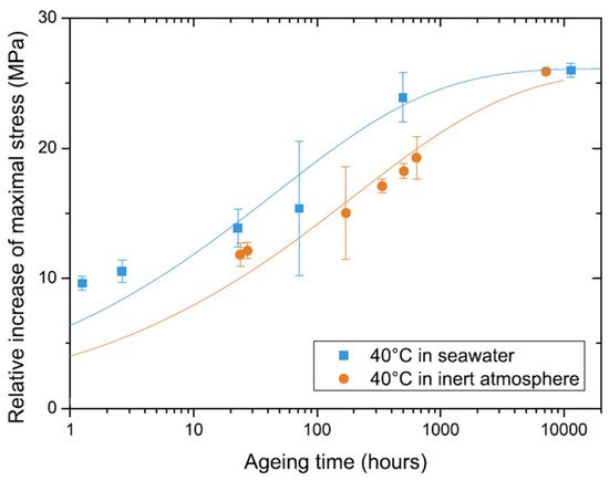
Figure 6. Strength vs. ageing time for amine-based epoxy conditioned in seawater up to saturation (wet) and in an inert atmosphere (dry). Adopted with permission from Ref. [96]. Copyright 2019 Elsevier.
Some authors correlate the material response with the time of any ageing process, e.g., caused by thermal or hydrothermal influence [46,55]. The time of a material exposure under specific conditions is considered as a factor affecting its relaxation behaviour. At the same time, the shift function in Equation (5) is related to this specific ageing time rather than temperature as in TTSP or moisture content in TMSP. For instance, the time–ageing time equivalence was applied to predict the viscoelastic behaviour of hydrothermally aged epoxy adhesive [46] and thermally aged PMMA [55]. Saseendran et al. [68] introduced the curing-time shift function to consider the curing history influence on the epoxy’s viscoelastic behaviour. The suggested approach combined with traditional TTSP is a powerful tool for predicting the long-term viscoelastic behaviour of partially cured polymer systems. However, the applicability of such ageing time-based approaches needs to be critically assessed due to the irreversible nature of ageing phenomena. Considering the cross-coupled influence of temperature and post-curing effects, a material needs to be classified as a thermorheologically complex material resulting in the development of more complex viscoelastic models and multistep procedures for generation of reliable master curves [55,68]. Some considerations on the curing-assisted chemical shrinkage and its effect on the viscoelastic behaviour of an epoxy system were reported by Böckenhoff et al. [35].
Temperature and time-related changes in the structure of polymers can lead to significant discrepancies between the time–temperature shift factors and master curves constructed based on the results of DMTA tests and traditional strain-controlled macrotests [34,111]. It is widely accepted that DMTA temperature and frequency scanning is an efficient approach, in terms of time and materials savings, for long-term predictions of the viscoelastic behaviour of polymer composites. In a recent study by Kontou and Spathis [111], the nonisothermal creep response of PMMA was predicted based on DMTA results. The authors introduced the energy barrier’s distribution density function determined from the experimental frequency-sweep data of the loss modulus. Once this function is determined, the fundamental time-dependent functions can be evaluated, and creep response can be effectively predicted. However, the approach has some limitations to the applied temperature and stresses to avoid the contributions of plastic strains. Another point resulting in discrepancies between the long-term predictions by different methods is related to a polymer’s physical ageing and after-cure effects during high-temperature accelerated DMTA tests or relatively long macrotests [34]. Duration of the former tests is generally in the range of tens of minutes, while the latter control tests can last for up to several months.
Guedes provided a comprehensive review of durability prediction methods of polymer matrix composites under static and fatigue loadings [9,75]. The lifetime predictions were critically assessed based on different failure criteria (rate theory of fracture, energy-based Reiner–Weissenberg criteria, fracture mechanics, Monkman–Grant).
3. Plasticity-Controlled Failure
Failure of polymers and other materials (e.g., metals, geomaterials, concrete) is associated with accumulation of (visco)plastic strains under loading. Creep failure testing is essential from the practical point of view for assessing the long-term static strength. Additionally, it contributes to understanding the mechanisms involved in the time-dependent deformation of the materials. The entire process of creep deformation can be divided into three stages: primary (transient), secondary (stationary), and tertiary (accelerated) creep (Figure 7). Primary creep is the viscoelastic region, where strain rate decreases with time and strain. During secondary creep, the strain rate reaches a constant steady plastic flow rate, which gradually accelerates (tertiary creep), eventually leading to strain localisation and failure [76,112].
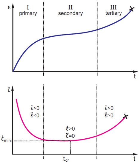
Figure 7. Typical creep curves: evolution of strain (top) and strain rate (bottom) with time.
Failure is an unstable process related to the microstructural specificity of a sample and testing conditions [31,80]; thus, failure predictions should be based on an extensive experimental data set and statistical analysis [113]. At the same time, in most applications, materials are exploited in the secondary creep regime, while tertiary creep is undesirable and considered the overshoot of the safety intervals [76]. Thus, many approaches consider the transition from the secondary to tertiary creep stage as a limiting factor or failure criteria defined by the strain rate minimum (Figure 7), for instance, the creep failure time model developed by Spathis and Kontou [31] and Monkman–Grant parametrisation [75,114] (see also Section 2.4).
Strain rate minima are determined from the strain rate vs. strain dependences called Sherby–Dorn plots [69,70,112]. As examples, Sherby–Dorn plots for glass-fibre reinforced isostatic polypropylene (iPP) [72] and carbon nanotube (CNT) reinforced polycarbonate [69] composites tested in uniaxial creep at 23 °C under various stresses are shown in Figure 8. It is seen that positions of strain rate minima increase with growing stress levels.
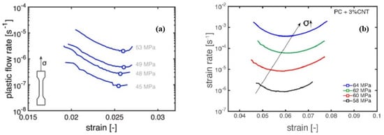
Figure 8. Sherby–Dorn plots for (a) glass-fibre reinforced iPP composites [72], and (b) polycarbonate/CNT composites [69], tested in uniaxial creep at 23 °C under various stresses.
A methodology for prediction of long-term failure under the plasticity-controlled mechanism has been proposed by Erp et al. for oriented polypropylene [70] and further validated in a series of studies of Govaert and coworkers for various engineering thermoplastic polymers [73] and their fibre reinforced composites [71,72] and nanocomposites [69]. The method is based on the “critical strain” concept and the Eyring thermal activation theory for viscoplastic flow. This enables the assessment of the stress and temperature dependences of plastic flow under creep loading by means of tensile tests at different strain rates.
The Eyring’s relationship between the plastic flow rate ε˙pl and the applied stress σ is given as follows [89]:
where ε˙0 is a rate factor, ϑ∗ is the activation volume, and kB is Boltzmann’s constant; other designations are the same as in Equation (3). Time-to-failure in the plasticity-controlled region can be estimated by calculating the total accumulated strain [69,70]:
where εpl is the viscoplastic strain at a certain time, ε˙pl is given by Equation (22). A criterion for failure is εpl=εcr, where εcr is the critical strain related to the onset of plastic strain localisation.
ε˙pl(σ,T)=ε˙0exp(−EaRT)sinh(σϑ∗kBT)
εpl(t)=∫t′0ε˙pl(σ,T,t′)dt
According to the time–stress equivalence and experimental observations, the creep failure time multiplied by the strain rate at failure ε˙f is constant for different applied stresses, i.e., ε˙ftf=const [115]. Taking into account considerations on the creep failure stages (Figure 7), the strain rate at failure ε˙f could be replaced by the minimum strain rate ε˙min, i.e.,
ε˙mintf=εcr
Going forward, Equation (24) is a special case of the Monkman–Grant relationship considered in the next section, Section 2.4.
It is worth noting that although εcr is usually smaller than the actual failure strain (see strain values at ε˙min in Sherby–Dorn plots, Figure 8), this phenomenological measure is reliable for predicting the time-to-failure of polymers [70].
Further, assuming that the state of deformation during secondary creep is identical to that obtained at the yield point σy in a constant strain rate test, one can write the following [70]:
tf(σ1)tf(σ2)=ε˙min(σ2)ε˙min(σ1)=ε˙pl(σy2)ε˙pl(σy1)
The replacement of ε˙min to ε˙pl in Equation (25) is beneficial from a practical point of view, since the experimental assessment of ε˙pl vs. σy is based on the data of constant strain rate tests at different strain rates, which is much easier and less time-consuming compared to creep failure tests resulting in ε˙min vs. σ dependences. A perfect correlation between the strain rate dependences of the yield stress determined in tensile tests and applied stresses in creep tests is demonstrated in Figure 9a for glass fibre reinforced thermoplastics [72]. According to Equation (24), the strain rate vs. time to failure follows a linear trend with a slope −1 (Figure 9b).
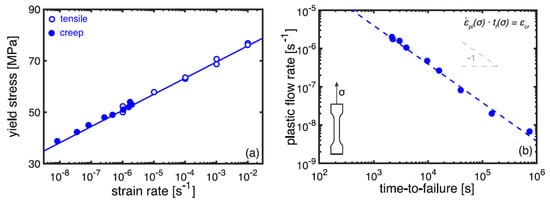
Figure 9. Strain rate dependencies of the yield stress in tensile tests and applied stress in creep tests (a) and a correlation between the plastic flow rate and time-to-failure according to Equation (24) (b) for glass fibre reinforced isostatic polypropylene composites [72].
The “critical strain” concept has also been verified for assessment of failure time of PA6 under the impact of temperature and humidity [74]. In addition, the method can be used as an effective tool for studying competition between two failure mechanisms in static loading and cyclic fatigue, namely plasticity-controlled and crack-growth controlled failure, respectively. Both mechanisms were effectively distinguished by comparing lifetimes for various thermoplastic polymer systems determined in creep and fatigue tests [71,72] (Table 1). “Critical strain” was independent of creep or fatigue loading under certain stress ratios. As applied to polymer nanocomposites, Pastukhov et al. demonstrated that adding carbon nanotubes into polycarbonate has a positive hampering effect on the plasticity-controlled failure. In contrast, the crack-growth-controlled regime has a negative accelerating effect [69].
Creep lifetime is strongly related to the accumulation of irreversible strains; thus, models for predicting their evolution are of great interest. The viscoplastic strain is expressed as nonlinear functions of stress, time, temperature, etc., e.g., Zapas–Crisman model discussed elsewhere [65,112,116,117]. Identification of multiple model parameters requires an extensive testing campaign that is often not justified in terms of costs. Simple, cost-effective methods with a minimum required amount of a priori known material parameters are advantageous for practical applications. In a recent study by Starkova et al. [80], a simple power-law relationship between the residual (viscoplastic) and the total creep strain was established (Figure 10):
where εvp is the accumulated viscoplastic strain measured as the residual strain in creep-recovery tests, C0 and n are material constants; n takes values in the range 0.7–2 and is equal to unity in the case of linear dependence between the residual and total creep strain [112,118]. The data were generalised for many polymers and composites reinforced with different types and amounts of fillers and tested under a wide range of stresses and temperatures. With increasing stress, loading time, temperature, or other external factors, one shifts forward on the curve εvp vs. εcreep, while increasing amounts of filler in host polymers (MWCNT in polypropylene in the present case) results in a shift down on the curve (Figure 10). Data representation in the form of Equation (26) is advantageous due to the implicit coupling of viscoelastic, viscoplastic, and damage-related strain components with no focus on the origin of irreversible effects. The results were consistent with known strain-rate-based modelling approaches [119,120].
εvp=C0(εcreep)n
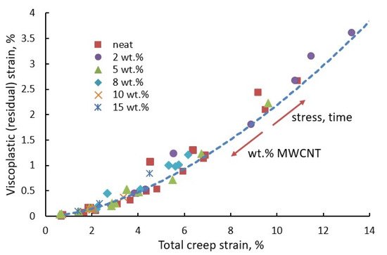
Figure 10. Residual recovery strain vs. total creep strain for polypropylene filled with different contents of MWCNT. Data obtained in creep-recovery tests under various loads and creep times; one point corresponds to one creep-recovery test. Data reproduced from [80].
4. Parametric Methods for Creep
Parametric approaches are methods through which the short-term creep-rupture data can be extrapolated using a time–temperature parameter. This concept is based on the assumption that all creep-rupture data can be superimposed to produce a single master curve: the stress vs. a parameter that combines time and temperature [114]. Long-term predictions are obtained based on this master curve constructed using available short-term measurements monitored in a few standard creep-rupture tests at different test temperatures and different stress levels. These extrapolation techniques were initially developed for metals and later validated for other materials, including polymers and composites [75,76]. It is worth noting that rupture can be defined by some limit value of strain, related to the safety criteria, or by actual rupture, depending on requirements set to a material.
According to phenomenological models, Larson–Miller and Monkman–Grant parametrisations are among the most used formulations due to their simple form and tractability. In the former method, originally derived from the Arrhenius relation, the Larson–Miller parameter (LMP) relates the creep rupture time at different temperatures under given stress as follows [57,76]:
where T is the temperature in Kelvin, tr is the creep rupture time, and CLMP is a material constant. CLMP is determined by fitting a line logtr vs. 1/T for a given stress level. Data for different temperatures in the axes stress vs. LMP fit on a common master curve (Figure 11) that could be linear [76] or fitted by a power law [57].
LMP=T(logtr+CLMP)
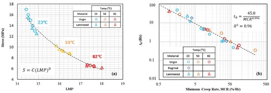
Figure 11. LMP master curve (a) and Monkman–Grant correlation tr vs. ε˙min (b) for HDPE under various temperatures [57].
The Monkman–Grant (MG) parametric method uses the minimum strain rate ε˙min as a key variable to assess the time to rupture tr. It is assumed that the mechanisms that control creep deformation and creep rupture are the same to a large extent. The Monkman–Grant relationship is given by the following relationship [57,75]:
where CMG is the Monkman-Grant parameter and β is a material constant. Log–log plot of tr vs. ε˙min forms a unified master curve for all temperatures (Figure 11), as it is demonstrated by the studies on HDPE [57], GFRP [75], and adhesive anchors [77] (Table 1). The practical advantage of the Monkman–Grant method, along with other strain-rate minimum based methods considered in Section 2.3, is that ε˙min can be measured at an early stage of a creep test well before the material’s end-of-life, thus reducing the time required to predict the long-term time to rupture.
CMG=tr(ε˙min)β
The Monkman–Grant relation is a special case of the general Voight’s relationship describing rate-dependent material failure, which is a basis of the well-known failure forecast method originally developed for landslide and volcanic eruption forecasts [119,120]. Corcoran and Davies [120] analysed creep as a positive feedback mechanism showing that an increase in strain leads to an increasing strain rate, which indicates damage and proximity to failure. According to Guedes’s considerations on failure predictions of GFRP [75], the Monkman–Grant equation is “built-in” in the Reiner–Weissenberg energy criteria and maximum stress work criteria.
Both Larson–Miller and Monkman–Grant methods might offer the possibility of long-term extrapolation if the same creep-deformation mechanism operates during the whole creep life. If the dominant mechanism changes, measurements made at high stresses would not allow the prediction of the low-stress behaviour. Then, constants used in Equations (27) and (28) become stress and temperature-dependent functions, and thus, more materials need to be tested and examined using these techniques to generalise their use. The Larson–Miller approach is valid for assessing both static and creep rupture time, while the Monkman–Grant method cannot be used to compare creep failure with static failure under constant strain or stress rate [75]. The Larson–Miller parametrisation can also be used for predicting the fatigue lifetime of composites (see Section 2.5.3).
5. Fatigue Prediction Methods
5.1. Factors Affecting Fatigue Damage
Fatigue failure of composites is challenging to analyse due to the heterogeneous and anisotropic nature of the material, as well as the complexity and interaction of many damage mechanisms. Numerous mechanisms can be identified for traditional FRP laminates: matrix cracking, fibre-interface failure, fibre fracture, fibre microbuckling, crack coupling, and delamination [121]. The damage mechanisms interact with each other and are characterised by different growth rates; thus, these are associated with different stages of fatigue. Three general stages are typically observed in conventional quasi-isotropic laminates [122,123]: cycling loading initiates the formation of microcracks and voids (first stage), which are further localised, causing minor damage (second stage) and finally promote macrocrack growth leading to an ultimate material failure (third stage). This continuous damage process leads to significant degradation of the mechanical properties such as the strength and elastic modulus. Thus, these parameters are generally used as a measure of damage [121,124,125,126,127].
Fatigue durability is affected by numerous factors, which can be divided into three major groups:
- (i)
-
Material related factors: fibre type and dimensions, matrix type, fibre volume content, reinforcement structure (unidirectional, multidirectional, woven, braided, spatially reinforced, etc.), laminate stacking sequence, etc.
- (ii)
-
Testing related factors: loading conditions (stress ratio, cyclic frequency, monotonic/variable frequency, axial/multiaxial loading, force/displacement-controlled loading), and environmental conditions (temperature, humidity, water/salt water, UV).
- (iii)
-
Manufacturing and storage-related factors: manufacturing process, inherent defects and voids, thermal or ageing pre-history, etc.
Slight variations in the design of novel composite materials or their operating and storage conditions result in extensive growth of experimental testing campaigns required to characterise fatigue durability and assess their lifetime [128]. Fatigue models reduce the number of tests necessary for long-term predictions of the behaviour of composites under cyclic loading. The essential initial step is understanding the damage mechanisms occurring in composites during fatigue.
Many empirical and theoretical models based on both global (homogeneous) and micromechanical (multiscale) formulations have been established to model and eventually predict different material systems’ fatigue life. These are comprehensively discussed and systematised in numerous review papers [121,126,129,130,131,132,133,134]. The traditional models are often used in conjunction with statistical data analysis [135,136,137,138,139]. The present section is not aimed to give an in-depth discussion of the fatigue models but point out the main differences in existing modelling approaches that are crucial for fatigue prediction under environmental impact.
5.2. Classification of Fatigue Models
Fatigue damage models may be assigned into different categories depending on their theoretical basis, “measurable” property, and structural levels of material involved in modelling [129]. There is usually no clear boundary between the categories, while categorisations are made mainly to highlight the role of the specific model in the development of subsequent models. Vassilopolous [130] reviewed the fatigue models for FRP in chronological order. Fatemi and Yang [131] categorised the reviewed theories and models into six categories: (a) linear damage rules, (b) nonlinear damage curve and two-stage linearization methods, (c) life curve modification methods, (d) approaches based on crack growth concepts, (e) continuum damage mechanics models, and (f) energy-based theories. Andersons [140] grouped the methods for fatigue prediction of composite laminates according to the structural level of material description: laminate, laminae, and fibre-matrix properties. Sendeckyj [141] introduced classification based on the fatigue criteria, namely four major categories: the macroscopic strength fatigue criteria, the residual strength and residual stiffness criteria, and the damage mechanism-based criteria. This classification with minor modifications has been further employed in numerous studies [121,142,143] and briefly justified within the following paragraphs.
Based on Sendeckyj’s formulation, the fatigue models for polymer composites can be divided into three major categories: (I) fatigue life models, (II) residual property models, and (III) progressive damage models (Figure 12).
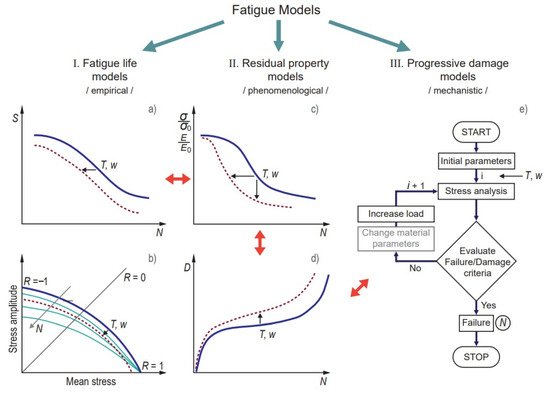
Figure 12. Classification of fatigue models and the principal ways for predicting the environmental impact (e.g., temperature T and water content w). Representative methods for fatigue analysis: (a) S–N curve; (b) constant life diagram; (c) residual strength/stiffness dependence on the number of cycles; (d) damage function; (e) flowchart of progressive damage analysis.
This classification consists of
(I) Fatigue life models (or empirical models) are based on the construction of the Wöhler S–N curves (Figure 12a), which provide information on the number of cycles (N) required to material failure under a given stress S and stress ratio defined as the ratio between the minimum and the maximum cyclic stress: R= σmin/σmax. Stress S may have different definitions: stress amplitude Sa = (σmax − σmin)/2, mean stress Sm = (σmax + σmin)/2, or normalised stress divided by a reference such as ultimate strength Su. Constant life diagrams (CLD), also called Goodman-type diagrams, are obtained by plotting Sa vs. Sm and presenting isolife lines with N=const, i.e., endurance limits (Figure 12b). Many examples of fatigue life models can be found in the literature [121,134]. Fatigue life predictions are commonly obtained by fitting a set of experimental data, in most cases by the Basquin-type power law equation [26,78,124]:
where A and B are fitting parameters found from the S–N line in log–log (or linear–log) scale as the intercept at N = 1 (A) and its slope (B). Equation (29), however, is limited in use for high cyclic fatigue. In contrast, in low cyclic and very high cyclic fatigue tests, deviations from the linear S–N dependence typically take place due to fatigue–creep interactions or self-heating phenomena, respectively. Nevertheless, these models are considered the primary engineering models for predicting fatigue failure of composites due to their simplicity and easy tractability. The main drawback of the S–N models is that they do not indicate the underlying failure mechanism; thus, they are only valid for a specific material under specific loading and environmental conditions. A lack of data generalisation requires extensive testing campaigns for sufficient material characterisation. Note that in low-cycle fatigue applications or materials with significant plastic deformations, S–N curve stress-life analysis can be replaced by the strain-life analysis, whose mathematical representation is similar to Equation (29) [144,145].
S=A(N)−B → logS=logA−BlogN
(II) Residual property models (or phenomenological models) measure the loss of macroproperty during cycling loading. They can be subclassified in (i) strength and stiffness degradation models and (ii) fracture mechanics-based or crack growth models. In the former models, an empirical function is defined for describing experimentally observed gradual degradation of residual strength (σ/σ0) or stiffness (E/E0) with respect to the number of cycles (parameters with subscripts 0 are related to the initial undamaged materials property). The rate of strength degradation is typically defined as a function of several factors:
dσdN=F(σmin, σmax, R…)
Different forms of this function are considered in numerous research studies and reviews [121,125,126,136,140,146,147,148]. Failure occurs when the residual strength equals the maximum cyclic stress. Under constant-amplitude stress conditions, Equation (30) integration results in the S–N curve dependence. Thus, the fatigue life model is, in fact, a particular case of the residual strength model. The strength-based models provide a simple and clear explanation of fatigue failure. However, these are not widely accepted within the engineering community due to the extremely high experimental cost of measuring the residual strength (due to a large number of destructive tests, material- and testing-related sensitivity, etc.) [136]. Nevertheless, the strength degradation approach is advantageous in many cases due to the ability to account for the effect of fatigue damage without the need for its detailed analysis cycle-by-cycle.
The damage rate usually characterises the loss of stiffness:
where D is the damage variable defined according to continuum damage mechanics as D=1−E/E0. The stiffness degradation models have been considered by numerous authors [121,127,149,150,151,152,153]. Contrary to the residual strength measurements, loss of stiffness presents much less data scatter and can be evaluated by nondestructive testing techniques, thus significantly reducing experimental costs for predicting fatigue durability of composites [140]. The residual stiffness and strength damage variables are also interrelated [154]. The limitation of the stiffness degradation model is the fact that it does not account for the different stages of composite damage mechanisms. For example, during the cyclic loading of off-axis laminates, initial stiffness degradation is caused by matrix transverse cracking while after that delamination and fibre failure occurs, which may have a different impact on stiffness degradation and residual life.
dDdN=F(σmin, σmax, D…)
The fracture-mechanics-based models describe the initiation and growth of cracks in composites caused by cyclic loading [122]. Mostly, delamination cracks are under interest, although off-axis matrix cracking and fibre/matrix debonding can also be introduced into micromechanical models [139]. These models can also be classified as mechanistic models. The fatigue failure analysis is done by means of crack initiation curves, which is similar to an S–N curve (Equation (29)) but instead of the characteristic cyclic stress, the maximum applied energy release rate Gmax is used:
where AG and m are material parameters. In the crack propagation phase, a power-law dependence, known as Paris law, is established between the crack growth rate da/dN and Gmax [71,123,139,155,156]:
where C and p are material parameters. The fracture-mechanics-based models explain failure mechanisms and damage development in composites, although the general failure analysis is done by the empirical approach.
Gmax=AG(N)−m
dadN=C(Gmax)p
(III) Progressive damage models (or mechanistic models) estimate the current state of material degradation through a set of measurable internal damage variables (e.g., transverse matrix cracks, delamination). Generally, these models combine the phenomenological models and the definition of a fatigue failure criterion [155,157]. The progressive damage models calculate the stress analysis at each cycle or number of cycles and then recalculate the stress and internal variables according to the specific failure criteria [123,154,157] (see the flowchart in Figure 12e). The latter is defined depending on the nature and interaction of damage mechanisms. Thus, these models are expected to provide a deeper understanding of the fatigue failure phenomenon. However, this is done at the cost of complex numerical calculations.
Damage, e.g., fibre break and debond propagation, changes the local stress distribution, and this stress varies over the fatigue life [139]. To account for this, the concept of cumulative fatigue damage is adopted to sum the damage accumulation at different stress levels. Miner’s rule, also known as Palmgren–Miner rule or the linear damage rule, is the simplest and therefore most popular damage accumulation rule [129]. It defines damage of a structure subjected to cyclic loading as the linear sum of the ratios between the ni of cycles applied to the structure and the Nfi of cycles that would cause fatigue failure of the structure on a given loading amplitude [158]:
where D is the damage variable, ni is the number of cycles at a given load amplitude and NFi is the number of cycles that would cause the failure of a part under the same load amplitude. Damage must remain lower than 1 to avoid failure.
D=∑iniNfi ≤1
This damage variable, as defined above, is clearly linear (Figure 13a). There are cases where it is useful to employ nonlinear damage laws to increase the damaging effect of low amplitude or high amplitude loading (Figure 13b,c). The damage parameter can be expressed through strength or stiffness changes that are correlated, e.g., by power-law dependence Dσ=(DE)b, where b is the material parameter [154]. The progressive damage models are based on the strength or stiffness degradation concept, while property changes are assessed cycle-by-cycle.
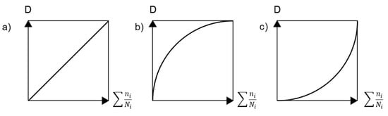
Figure 13. Damage accumulation types: (a) linear, (b) hyperlinear, (c) hypolinear.
5.3. Fatigue Prediction under the Environmental Impact
Variations in temperature, the humidity of ambient air, and other environmental factors contribute to the damage accumulation and determine the fatigue life of composites. Environments typically degrade the matrix material and the fibre/matrix interface, which are crucial for triggering further damage mechanisms and general fatigue response of FRP [26,132,156,159,160]. Reliable durability forecasts require a tremendous amount of highly undesirable testing costs. At the same time, studies on the fatigue of composites under environmental ageing are fragmentary and mostly experimental, while modelling approaches meet conflicting requirements of versatility and minimal experimental efforts needed for their validation. This implies the need to overview and systematise fatigue prediction methods under environmental impacts. Some of these methods are reviewed within the current section.
The predictive fatigue methodologies can be divided into several categories related to the classification used in Section 2.5.1 and the “property of interest” depending on how an environmental factor’s action is introduced into the model. Elevated temperature (T) and absorbed water (w) reduce fatigue lifetime of polymer composites that appears in a shift and/or change of slope of S–N curves (Figure 12a), narrowing and transformation of constant life diagrams (Figure 12b), decreased residual properties (Figure 12c), and accelerated damage (Figure 12d). The influence of accelerated factors can be accounted for by phenomenological approaches, e.g., TTSP, assessing global fatigue behaviour, and mechanistic models considering material damage on its different structural levels and updating the damage state until failure (Figure 12e). The current study is focused on phenomenological models due to their simplicity and availability for practical applications. Fatigue prediction methods can be grouped as follows:
(I) Construction of S–N master curves according to TTSP, similarly as it is done for viscoelastic properties of polymers (Section 2.2.1). The fatigue master curves are constructed based on Equation (29) and using the reduced frequency f′ and the reduced time to failure t′f concepts (Equation (5)):
t′f=Nf′=tfaT
For different temperatures, S–N curves are horizontally shifted to the reference S–N curve, typically obtained under room temperature. An example of S–N master curves constructed from four-point bending tests at different temperatures for dry and wet GFRP samples is shown in Figure 14 [26].
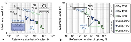
Figure 14. S–N master curves for dry and conditioned GFRP (a) and superimposed environmental master curve with the definition of equivalent temperature (b) [26].
The shift factors are determined by the Arrhenius relationship (Equation (9)) with the activation energies different for temperature ranges above and below the polymer’s Tg. Under the coupled influence of temperature and absorbed water, the water effect, related to both accelerated viscoelastic response of the polymer matrix and triggering additional damage mechanisms, is taken into account via the modified temperature shift functions. This methodology has been used by Gagani et al. [26], Zhou and Wu [133], and Fatemi et al. [146,161].
(II) Accelerated methodology developed by Miyano and Nakada et al. [42,53,90,162] assumes the same failure process for the accelerated loading history under elevated temperature and introduces three main hypotheses (Figure 15):
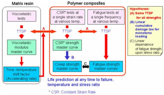
Figure 15. Formulation of accelerated testing methodology by Nakada and Miyano. Adapted with permission from Ref. [53]. Copyright 2009 Elsevier.
(A) The same TTSP is applicable for all strengths determined in constant strain-rate, creep, and fatigue tests. The temperature effect is solely associated with the viscoelastic properties of a polymer matrix; thus, the time–temperature shift factors are assumed to be the same for the polymer and composite and independent of a loading regime.
(B) Linear cumulative damage law for monotonic loading predicts creep strength from the static strength master curve.
(C) Linear dependence of the fatigue strength upon stress ratio applies to predicting fatigue under an arbitrary stress ratio.
The proposed methodology has been successfully validated for different FRPs, loading conditions, and ageing factors (temperature and moisture) [42,53,67,90,162]. Overall, the culminating point of this method also consists in the construction of S–N master curves, albeit at lower experimental cost than the previous method. Recently, authors proposed the advanced accelerated testing methodology for unidirectional CFRP introducing statistical assessment of the strength and a fatigue degradation parameter based on matrix viscoelasticity [43,135].
(III) Larson–Miller parametrisation for fatigue lifetime and construction of the master curves from data obtained at different temperatures, similar to the procedure for creep tests described in Section 2.4 (Table 1). According to methodology introduced by Eftekhari et al. [78,79], the fatigue stress amplitude can be expressed similarly to Equation (27):
where A’ and B’ are material parameters. The Larson–Miller parameter for fatigue (LMPf) is defined as:
where tf is time to failure in fatigue test in hour, and CLMPf is a material constant determined by fitting lines logtf vs. 1/T for a given stress amplitude. The time to failure is converted to cycles to failure N using the test frequency: tf=N/(f×3600).
S=A'(LMPf)B'
LMPf=T(logtf+CLMPf)1000
Equations (36) and (37) are used to relate the stress amplitude, temperature, cycles to failure, and frequency for each material. The Larson–Miller fatigue master curves for polypropylene, neat (PP) and reinforced with talc (PP-T), and glass fibres (PP-G), are shown in Figure 16 [78]. Parameters CLMPf were found to be independent of the stress ratio R, while B’ varied slightly with R increase.
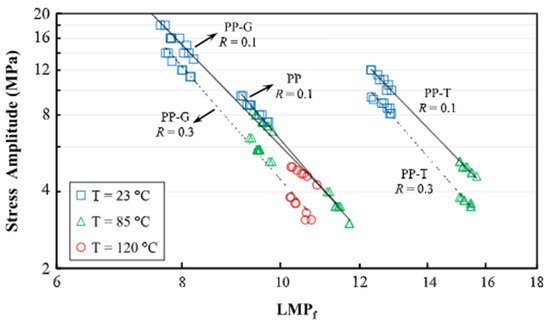
Figure 16. Larson–Miller master curves for polypropylene (PP), neat and reinforced with talc (PP-T), and glass fibres (PP-G) at R = 0.1 and 0.3. Adapted with permission from Ref. [78]. Copyright 2016 Elsevier.
(IV) Normalisation of the characteristic stress of the fatigue models, e.g., stress amplitude in Equation (29) or residual strength in Equation (30), to the ultimate strength of an aged material rather than a pristine one: Such “normalised” S–N curves at different temperatures or ageing states of material are superimposed on each other. This observation comes from the fact that temperature (water) affects only the properties of a polymer matrix. At the same time, damage mechanisms under static and cyclic loadings of both the pristine and aged material are believed to be the same. The same hypotheses are used in the accelerated methodology by Miyano and Nakada [53].
Chamis and Sinclair [163] proposed a generalised empirical relationship for prediction of fatigue lifetime of hygrothemally aged graphite-fibre/epoxy-matrix composites:
where Su0 is the reference initial static strength at the reference temperature T0, T is the test temperature, and Tg0 and Tgw are the glass transition temperature of the matrix in the dry and moisture saturated (wet) state, respectively; other parameters are the same as in Equation (29). Other authors modified Equation (38) to apply to thermoplastics by replacing glass transition temperatures to the melting [164] or other characteristic temperatures [165]. The first term in Equation (38) is associated with the constant A in Equation (29) and is related to the actual ultimate stress Su of the material at a given temperature and moisture content. Data plotted as S/Su vs. logN fit on a common dependence.
S=Su0(Tgw−TTg0−T0)1/2−BlogN
The S–N “normalisation” is employed in numerous studies, e.g., [133,146,161,164,165,166]. It is simple, predicts conservative values, and should be adequate for preliminary designs. This method is often interrelated with the strength degradation concept described in the next paragraph.
(V) Modelling S–N curves and the residual strength and stiffness by applying known models (Section 2.5.2) with temperature (or other environmental factors) dependent parameters: Such prediction methods can be based on empirical or physical considerations. The model parameters are determined by common fitting procedures, resulting in extensive and costly experimental testing. Figure 17 shows constant life diagrams for plain-woven CFRP aged in seawater for different times [167]. These were calculated based on the fatigue life prediction model using Basquin’s law and strength degradation model of Epaarachchi and Clausen. It is seen that environmental ageing resulted in lowering surface area under isolife lines indicating the decreased endurance limits of the material.
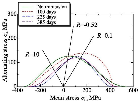
Figure 17. Constant life diagrams for plain-woven CFRP aged in seawater for different times. Adapted with permission from Ref. [167]. Copyright 2019 Elsevier.
Although these approaches can contribute to understanding the damage mechanisms under the environmental impact, these are characterised by limited versatility since all the fitting parameters are specific for a given material only. Modelling of fatigue properties by this methodology has been used by Tang et al. [151], Khan [152], Cormier et al. [136], Mivehchi et al. [149], Koshima et al. [167], Eftekhari and Fatemi [78], Amjadi and Fatemi [166], Prabhakar et al. [145], Solfiti et al. [168], and Acosta et al. [169]. The results are summarised in Table 2 regarding the environmental factors, material and testing parameters, and general concepts employed in modelling. Some alternative approaches for predicting fatigue lifetime under the influence of environmental factors are presented in [102,137,156,160].
Table 2. A condensed list of recent works modelling fatigue under environmental impacts (T and w are associated with temperature and water effects, respectively).