1. Introduction
Chemical process accidents have become a critical threat to sustainable development in our society. With the newly proposed carbon peaking and carbon neutrality goals, governments have strengthened the supervision on production safety, including establishing regulations and carrying out technical training. However, safety accidents still occur every year, resulting in major losses of property and human lives
[1][2][1,2]. According to numerous statistical analysis studies on chemical accidents, it can be concluded that human error is the main cause of chemical accidents
[3][4][3,4]. Although distributed control systems (DCS) have been widely applied in the chemical industry, it is still difficult for operators to detect abnormal process deviations and make proper decisions to eliminate them at an early stage due to the increasing scale of chemical production and equipment complexity. The operators can only focus on a few key variables out of a large number of process variables in DCS, and unnecessary alarms can be quite overwhelming without an effective fault detection and diagnosis system. Therefore, the emergence of process monitoring technology is crucial and necessary in the chemical industry.
Process monitoring technology has been developed as a useful tool to assist operators to ensure product quality and production safety. Process monitoring can be implemented in two steps, fault detection and diagnosis (FDD). Fault detection aims at determining whether the process is operating under normal conditions, and fault diagnosis works after a fault is detected to determine the root cause of the fault. Taking advantage of the wide application of DCS, massive historical data, which contain internal process operation mechanism information, could be obtained, making data-driven process monitoring methods a popular research focus, especially for industrial processes whose mechanistic models are hard to build
[5]. In the last 20 years, process monitoring technology has been developed to be an important and indispensable branch of process system engineering (PSE)
[6][7][6,7]. Comprehensive reviews of process data analytics and its application on process monitoring have been provided and discussed. In Chiang’s work in 2001, traditional multivariate statistical methods were introduced and compared based on their performance on process monitoring results of the Tennessee Eastman process (TEP)
[8]. In 2003, process history-based methods were reviewed and classified as an important type of process fault detection and diagnosis in a series of reviews by Venkatasubramanian
[9][10][11][9,10,11]. Qin made a deep survey on the advanced development of principal component analysis (PCA) and partial least squares (PLS)-based process monitoring methods
[12]. Reis and Gins discussed the industrial process monitoring issues in the era of big data from the perspectives of detection, diagnosis and prognosis
[13]. Severson et al. provided perspectives on progress in process monitoring systems by summarizing methods for each step of the process monitoring loop over the last twenty years
[14]. Ge introduced the framework of industrial process modeling and monitoring and reviewed data-driven methods according to various aspects of plant-wide industrial processes
[15]. Qin and Chiang presented the current development of machine learning and artificial intelligence (AI)-based data analytics and discussed opportunities in AI-based process monitoring
[16].
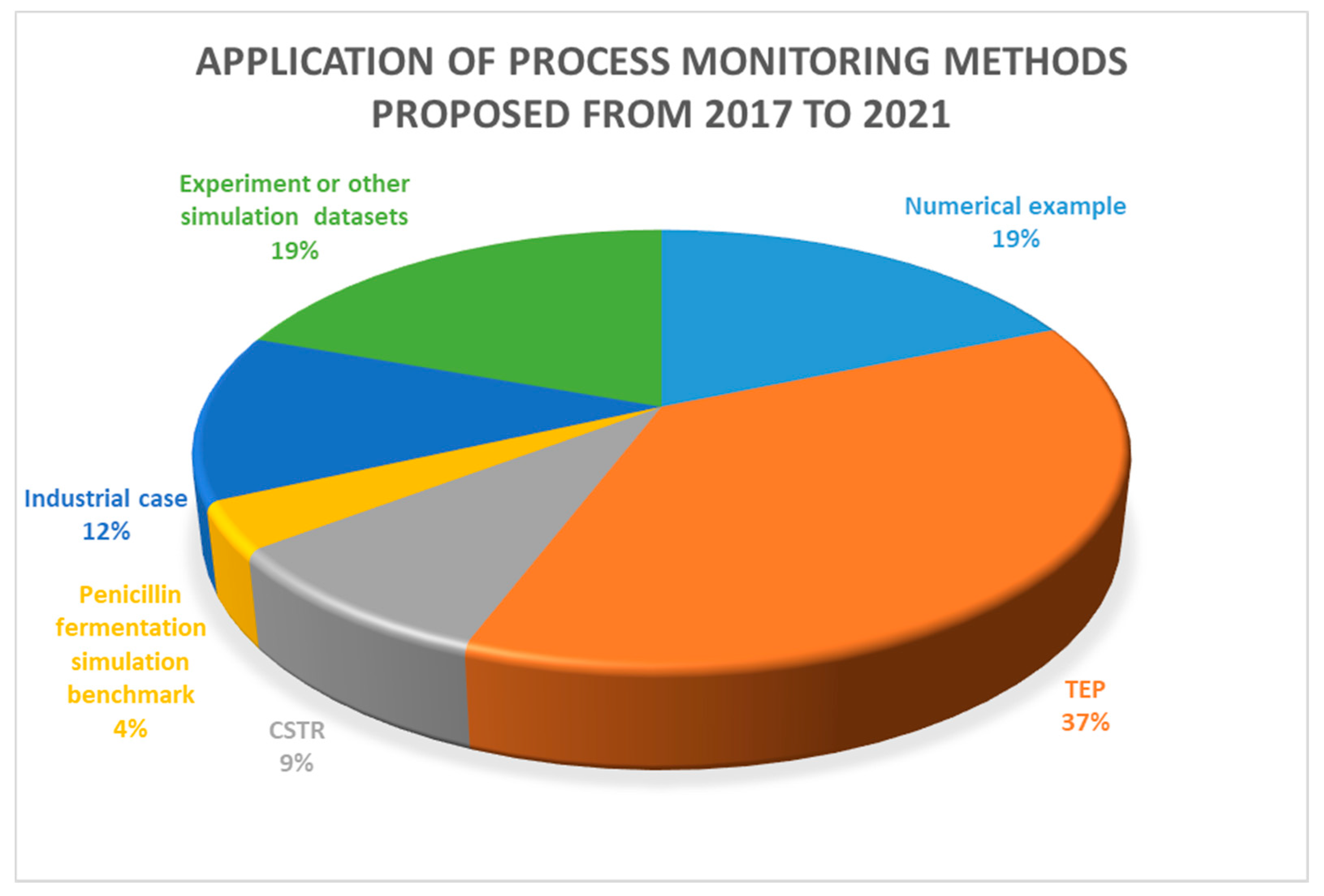
In recent years, with the popularity of the notion of industry 4.0 and the digital factory, data-driven process monitoring technologies have gradually attracted attention from industry. Unlike simulated data, industrial process data show more complex characteristics due to various practical operating conditions, which provides a huge challenge to industrial process monitoring. Figure 1 provides a statistic regarding the publication of proposed process monitoring methods from 2017 to 2021. This statistic was generated from the Web of Science by searching the keywords, “chemical process monitoring” and “data-driven”.
Figure 1. A statistic on the application of process monitoring methods.
A statistic on the application of process monitoring methods.
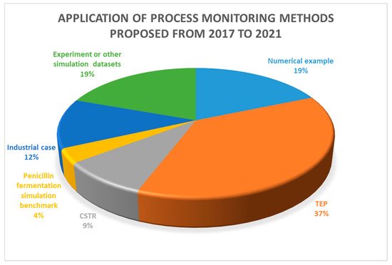
It can be seen that most proposed data-driven process monitoring methods were applied to simulated cases, such as numerical examples, TEP, continuous stirred tank reactor (CSTR), and penicillin fermentation simulation benchmarks, and only 12 percent of the studies were applied to practical industrial processes, indicating the huge difficulty in industrial process monitoring. Process monitoring methods that achieve good performance in simulation processes cannot be directly applied to industrial processes, because there are significant differences between practical industrial data and simulation data. Simulation process data are generally simulated under a single ideal operating condition, while industrial process data show complex characteristics due to various factors in practical production, as summarized in Figure 2. Industrial processes are not limited to a single operating condition, and characteristics of normal operating conditions also vary with different processes, which brings great challenges to the monitoring of industrial processes. On the other hand, it also indicates that industrial process monitoring can be well implemented if the normal operating conditions can be correctly defined and the characteristics of the normal operating conditions data can be effectively and completely extracted.
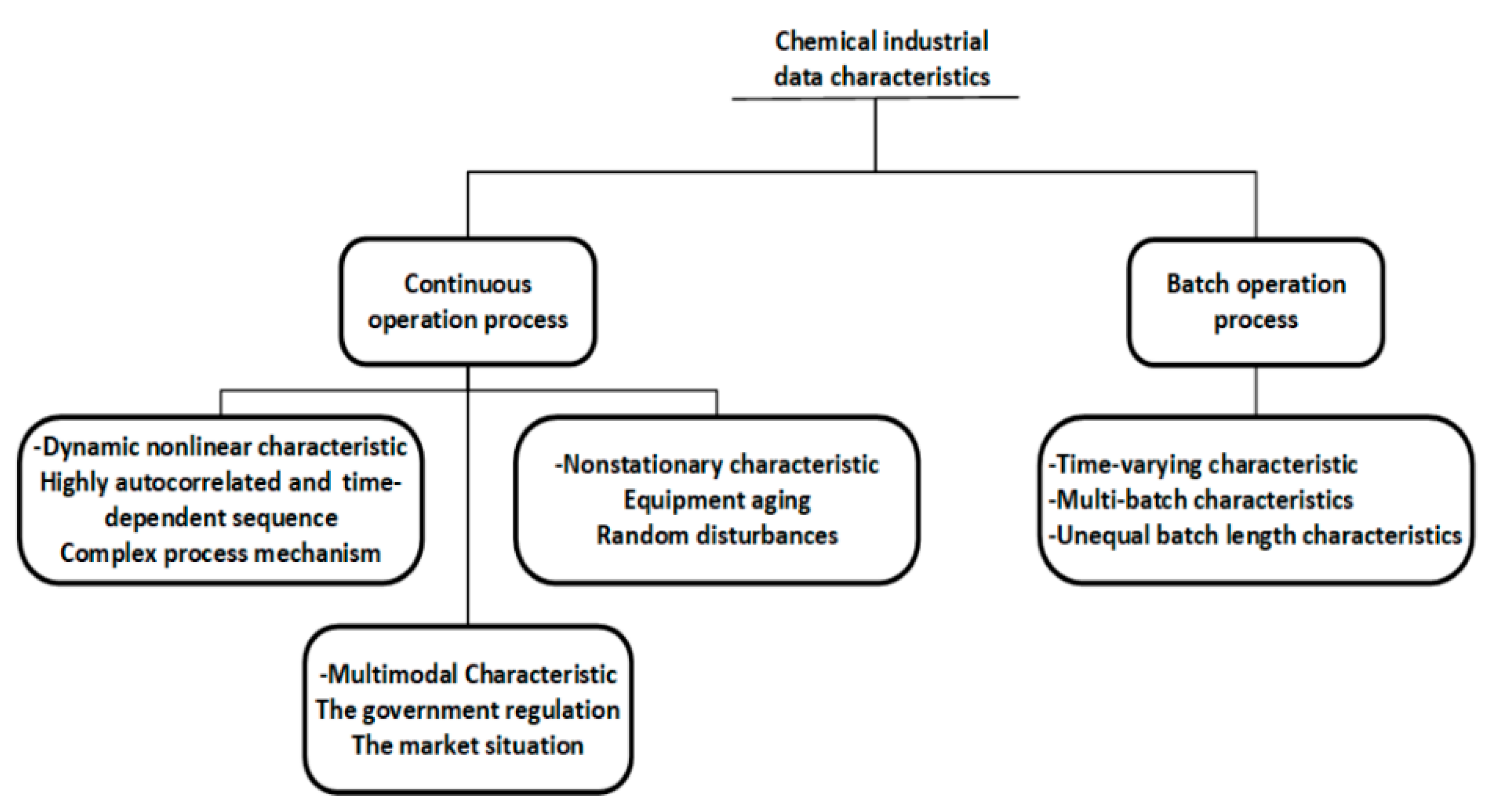
Figure 2. The characteristics of data from the chemical process industry.
The characteristics of data from the chemical process industry.
2. Data-Driven Process Monitoring
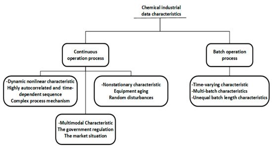
In this section, a data-driven process monitoring framework is presented from the perspective of defining normal operating conditions, data preprocessing, feature extraction, monitoring statistics, and fault diagnosis. The flow diagram of the data-driven industrial process monitoring framework is shown in Figure 3. Common methods applied to these key procedures are presented in each corresponding subsection.
Figure 3. Data-driven industrial process monitoring framework.
Data-driven industrial process monitoring framework.
2.1. Definition of Normal Operating Conditions
Different from commonly used simulation processes, such as CSTR and TEP, there are usually multiple complex operating conditions existing in industrial processes. In the academic field of process monitoring, the performance of the newly proposed method can be easily tested by comparing the process monitoring results using fault datasets, when a novel feature extraction method is proposed to extract the common feature of normal datasets and calculate the monitoring statistic. However, in industrial applications, the normal operating conditions and fault conditions are usually not so clearly distinguished as those in the simulation processes. The definition of normal operating conditions and the labelling of data are usually the most important and time-consuming tasks in building an industrial process monitoring model. With the increasing scale of modern industrial processes, huge historical datasets with high dimensionality are available, while the information for upcoming process situations is poor. Various types of random variations and unexpected disturbances are mixed up in the large amount of historical operating data. If these normal random variations are not fully captured when training a process monitoring, a large number of false alarms will be caused during online monitoring. On the other hand, if the unexpected disturbances in historical data are included in offline modeling, these kinds of abnormal conditions will be regarded as normal, resulting in alarm missing for real faults. Therefore, it is important to effectively separate abnormal disturbances from normal random variations. A certain process internal mechanism for information needs to be incorporated to help characterize data features under normal operating conditions. More importantly, it is necessary to consider the complex data characteristics in industrial processes. Among them, the multimode characteristics and nonstationary characteristics should be considered in the definition of normal operating conditions, these are analyzed in the following sections.
2.1.1. Multimode Characteristics
In industrial processes, production load is frequently adjusted due to fluctuations in the market price of the product and the upgradation of government regulations, especially in the context of carbon emission restrictions. Therefore, data in actual production often display multimode characteristics, which could be defined as at least one variable that does not follow a single steady operating condition due to various changes in production loads, feed flow, and set points
[17][18][17,18]. However, traditional statistic process monitoring models are established under the assumption that the process is operated at a single stable working point. When the operating condition is switched, the mean and variance of the data change significantly, and massive false alarms will be triggered, which can be categorized to multimode continuous process monitoring. In industrial scenarios, future modes are hard to estimate and are usually not available in historical datasets.
At first, data from multiple operating conditions cannot be simply integrated into one single training dataset, because the normal working point determined in this way is just an average of different operating conditions. At the same time, data associated with abnormal transitions between normal operating conditions may also belong to the assumed normal data range, which will affect the early identification of abnormal process deviations. Another challenge is that the operating conditions contained in training data will not cover all possible situations in actual production. Even if a corresponding model is established for each normal operating condition, when a brand-new operating condition appears, it will still be mistaken as a fault by such methods. In addition, the consideration of the transition states is inevitable since the switching of operating conditions cannot be completed instantaneously. The data characteristics in transition states are significantly different from steady states, as the mean of certain variables keeps changing until a new operating condition is reached. It is difficult to extract the common features of transition states, and the monitoring of transition states is the most critical challenge in multimode process monitoring.
2.1.2. Dynamic and Nonstationary Characteristics
In addition to multimode characteristics, different types of dynamic and nonstationary characteristics caused by various factors need to be considered in the definition of normal operating conditions. The concept of “dynamic” comes from process control and monitoring in PSE, and the concept of “nonstationary” is mostly defined in the field of time series analysis. Both “dynamic” and “nonstationary” can be considered as the time-variate nature of the variables in the process. In the category of process monitoring and fault diagnosis, the dynamic characteristics are obtained because sequences of certain variables are highly autocorrelated due to internal mechanisms and the response of control systems. Moreover, nonstationary characteristics are also reflected in practical production due to equipment aging, and random disturbances in process or environment. Resulting from the existence of these complex data characteristics, the means and variances of the variables are time-varying even in a single normal operating condition, particularly in a batch process. The time-varying characteristics violate the assumption of traditional multivariate statistic process monitoring that the process is time-independent, and therefore, limit the application of industrial process monitoring. In industrial practice, these time-varying characteristics caused by process dynamics and non-stationarity shall be defined as normal conditions, otherwise they will be regarded as process faults in real time monitoring, resulting in massive false alarms. In addition, minor abnormal changes that happen at the early stage of certain faults can be buried by these time-varying characteristics, which also should be considered when defining the range of normal operating conditions.
2.2. Data Preprocessing
Data preprocessing is a relatively straightforward but indispensable step in process modeling. There are two main purposes of data preprocessing, data reconciliation and data normalization.
During the process of data acquisition and data transmission, there will inevitably be missing values and outliers due to mechanical problems with data acquisition equipment and sensors. Data reconciliation technology is designed to deal with these problems through data removal or data supplement. When most variables at a measurement point are missing, these samples can be deleted, and if a small number of variables are missing, various data processing methods can be used to supplement the data. The simplest way is to supplement the current value with the value collected at the last moment or the average value of the previous time period. If there is a certain conservation relationship between the missing variables and other variables, the missing value can be supplemented through mass balance, energy balance, etc. To further improve the accuracy of data supplement, soft sensing technology can be applied to build regression models for missing values using historical data. The missing values can be replaced by predicted values through the regression relationship between other measurements and the missing measurements.
After the missing values have been effectively supplemented and outliers have been properly dealt, data normalization should be applied to balance the contribution scale of each variable before modeling. The most commonly used data normalization method, z-score normalization, aims to scale data samples to zero means and unit variance. Z-score normalization is suitable for processing normally distributed data and has become the default standardized method in many data analysis tools, such as PCA, and statistical product and service software (SPSS). Min-max normalization, logarithmic function conversion and logistic/SoftMax transformation are also commonly used data normalization methods. Different data normalization methods have various effects on the results of the model, but there is no general rule to follow in the selection of data normalization methods. In industrial process monitoring, data normalization methods can be selected according to the characteristics of process data and monitoring algorithms. In most cases, industrial data conform to a normal distribution and Z-score normalization is the most reliable method. When the process is highly nonlinear, logarithmic function conversion and kernel functions transformation should be considered. Furthermore, data expansion and batch normalization need to be implemented to unfold three-dimensional data into two dimensions and normalize data in different batches. The criterion to pick a proper data preprocessing method is decided by the requirement of feature extraction. Usually, data preprocessing is considered together with feature extraction. A summary of different data preprocessing methods is shown in Table 1.
Table 1.
A summary of data preprocessing methods.
| Data Preprocessing Methods |
| Data Reconciliation |
Data Normalization |
| Data removal; Data reconciliation with mass balance, energy balance; Data reconciliation with soft sensor technology |
Z-score normalization; Min-max normalization; Logarithmic function conversion; Logistic/SoftMax transformation; Kernel functions transformation; Data expansion |
2.3. Selection of Feature Extraction Method
Feature extraction is the problem of obtaining a new feature space through data conversion or data mapping. When sufficient training data from normal operating conditions have been selected and normalized, a proper feature extraction method should be applied to project or map the data into a low-dimensional feature space where most of the information from the original data can be retained. For example, the traditional statistic method, PCA, is applied to transform a set of originally correlated variables into a set of linearly uncorrelated variables, which are called principal components, through orthogonal transformation.
Based on the characteristics of data under normal operating conditions defined and analyzed in previous steps, corresponding feature extraction methods should be selected for modeling. For a simple linear process in which data are normally distributed, traditional PCA or PLS can be applied for feature extraction. If the process data do not conform to Gaussian distribution, methods that do not require assumptions about the distribution of the training data, such as independent component analysis (ICA) and support vector data description (SVDD), can be selected for feature extraction. When the process variables are highly nonlinear, kernel-based methods or neural network-based methods can be applied to extract process nonlinearity by nonlinear mapping. To extract process dynamic characteristics, time series analysis and autoregressive tools can be included in feature extraction methods. When dealing with more complex data characteristics in nonstationary processes, multimode processes and batch processes, more complicated feature extraction procedures need to be proposed by extracting the common normal trends in complex data features, and sometimes even a combination of multiple methods is required. A simple summary of different feature extraction methods for process monitoring is shown in
Table 2. A detailed review of feature extraction methods for various industrial process data characteristics is provided in
Section 3. Once the feature extraction method has been determined, the model needs to be trained and a corresponding statistic and its confidence interval should be constructed for fault detection. An introduction to monitoring statistics will be presented in the next section.
Table 2.
A summary of commonly used feature extraction methods.
| Methods |
Usage |
| PCA/PLS |
Linear Gaussian process monitoring |
| ICA/SVDD |
Non- Gaussian process monitoring |
| Kernel-based methods/neural network |
Nonlinear process monitoring |
| Dynamic PCA/PLS |
Dynamic process monitoring |
| Common trends analysis/cointegration |
Nonstationary process monitoring |
2.4. Monitoring Statistics
Feature extraction methods can only be applied to obtain a mapping or projection direction to transform the original data into a feature space, but it cannot be directly used to monitor the change in operating conditions
[19]. The construction of monitoring statistics is required for fault detection. Monitoring statistic is a measure of the distance between the measurement point and the original point in the feature space. Distance indicators have been widely used in constructing monitoring statistics, such as Euclidean distance and Mahalanobis distance. Typically,
T2 statistic is calculated to measure the variations in principal component subspace using Mahalanobis distance. Considering data under normal operating conditions following a multivariate normal distribution, the
T2 statistic can be regarded as an
F-distribution, and the control limits can be determined at different confidence levels
[20]. When the data do not conform to normal distribution, the control limits of
T2 statistic will not be reliable
[12]. In this case, the squared prediction error (SPE) statistic calculated based on Euclidean distance generally performs better to measure the projection on the residue subspace. The control limits can be obtained by approximating SPE statistics to a normal distribution with zero mean and unit variance
[21]. With the development of feature extraction technology, many novel monitoring statistics have been proposed accordingly. In moving PCA, a novel monitoring statistic is proposed to measure the difference in the angle of principle components between the current operating condition and the reference normal operating conditions
[19][22][23][19,22,23]. The difference in the probability distribution of data can also be applied as a monitoring statistic. Kano et al. proposed a process monitoring method by monitoring the distribution of process data, and therefore a dissimilarity index is introduced to quantify the difference in distribution between two sequences
[24]. As a common measure of the similarity between two probability distribution functions, Kullback–Leibler divergence (KLD) was introduced by Harrou et al. as a fault decision statistic to measure the variations of residues from PLS
[25]. Zeng et al. developed statistics based on KLD to measure variations in the probability distribution functions of data using a moving window
[26]. In the work of Cheng et al., negative variational score is derived from KLD as a novel statistic to monitor the distribution probability of data in probability space
[27].
To simplify the fault detection, multiple monitoring statistics can be combined and integrated into a single statistic. Decision fusion strategies are usually applied to fuse results from various methods to combine their strengths
[28]. Raich and Cinar proposed a combined statistic by introducing a weighting factor to the
T2 statistic and the SPE statistic
[29]. Yue and Qin also proposed a new statistic combing the
T2 statistic and the SPE statistic, but the control limits are constructed using the distribution of quadratic forms rather than using their respective thresholds
[30]. Different from a simple combination of the
T2 statistic and the SPE statistic, in the work of Choi and Lee, the
T2 statistic and the SPE statistic are combined into a unified index from the estimated likelihood of sample distribution
[31]. Another widely applied fault decision fusion method is Bayesian inference, by which an ensemble probabilistic index can be generated from multiple monitoring statistics
[32]. Moreover, SVDD has also been reported in multiblock methods to integrating monitoring statistics of multiple sub-blocks for plant-wide process monitoring
[33]. Based on the fusion of multiple monitoring statistics, variations in each feature space or sub-block could be comprehensively measured with a single statistic, which significantly simplifies the monitoring of process operating conditions and the shortcomings of each statistic could be overcome to a certain extent and an objective process monitoring result could be obtained. A summary of different types of statistics for process monitoring is shown in
Table 3.
Table 3.
A summary of different statistics for process monitoring.
| Process Monitoring Statistics |
| Distance-Based Statistics |
Probability Distribution-Based Statistics |
Other Statistics |
| Mahalanobis distance: | T2 | statistic; Euclidean distance: SPE statistic |
Kullback–Leibler divergence; Negative variational score |
Distribution of process data; Angle of principle components; Fault decision fusion strategy |
2.5. Fault Diagnosis
After the monitoring statistics calculated from real time data exceed their thresholds determined from offline modeling, it is critical to isolate the root cause of the fault through fault diagnosis. Fault diagnosis includes two consecutive steps: identification of fault variables and analysis of fault propagation path. The identification of fault variables aims to find out which variables are beyond their normal ranges and how much they contribute to the fault. The challenge is that the fault can be rapidly propagated from root variable to other variables with mass transfer and heat transfer, etc. A large number of variables will be identified and the variable with the largest contribution to the fault may not be the root cause, but just a result caused by the fault. Therefore, the fault propagation path among these identified fault variables needs to be further analyzed. If causal reasoning among these variables could be obtained, the fault propagation could be displayed in a network diagram and then the real root cause of the fault could be located. The acquisition of causal reasoning models among process variables has always been a challenge. Especially as industrial processes become more and more complex, variables are highly correlated with each other, and the causal logic among process variables may change due to the response of the control systems, which makes it difficult to capture the real time causal correlations among process variables.
Generally, fault diagnosis has an inseparable connection with fault detection. The fault variable’s isolation is usually realized on the basis of the fault detection model. For example, the fault diagnosis is implemented by finding the value of which variable exceeds its set point and which is determined offline for fault detection. In addition, fault variables identified in contribution plots are obtained by calculating their degree of deviation in corresponding feature spaces, which are defined by fault detection methods.