Your browser does not fully support modern features. Please upgrade for a smoother experience.
Please note this is a comparison between Version 2 by Vivi Li and Version 1 by Monica Berrondo.
Driven by its successes across domains such as computer vision and natural language processing, deep learning has recently entered the field of biology by aiding in cellular image classification, finding genomic connections, and advancing drug discovery. In drug discovery and protein engineering, a major goal is to design a molecule that will perform a useful function as a therapeutic drug. Typically, the focus has been on small molecules, but new approaches have been developed to apply these same principles of deep learning to biologics, such as antibodies.
- antibody
- antigen
- machine learning
- deep learning
- neural networks
- binding prediction
- protein–protein interaction
- epitope mapping
- drug discovery
- drug design
1. What Is Deep Learning?
Deep learning is a subset of machine learning, concerned with algorithms that are particularly capable of extracting high level features from raw, low level representations of data. An example of this is an algorithm which extracts object curvature or depth from raw pixels within an image. Deep learning algorithms generally consist of artificial neural networks (ANN) with one or more intermediate layers. The intermediate layers of an ANN make the network “deep” and can be considered responsible for transforming the low-level data into a more abstract high-level representation. Each layer of the network consists of an arrangement of nodes, or “neurons”, which each take as input a set of weighted values and transform them into a single output value (usually by summing the weighted inputs). The resulting values are then passed on to nodes in subsequent layers. The input values for the first layer are chosen by the practitioner or model architect. In a biochemical context, these features can be hand-crafted values such as a protein’s volume, or lower-level values such as an amino acid sequence. In a “deep” network, the outputs of the first layer are passed through one or more intermediate layers before the final output layer which produces the final result. The intermediate layers allow the network to learn non-linear relationships between inputs and outputs by extracting successively higher level features and passing them along to subsequent layers (Figure 31).
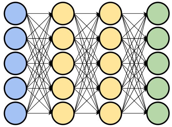
Figure 31. A representation of a deep learning neural network. Input layer in blue, output layer in green, and intermediate layers in yellow.
In order for a neural network to transform an input into a desired output, it must be “trained”. Training a neural network happens by modification of the weights of the connections between nodes. In a “fully connected” network each node is connected to each node in subsequent layers. The output values from the nodes of the preceding layer are passed along weighted connections to the nodes of the subsequent layer. These weights of the connections are typically initially randomized, and as the network is trained, corrections are made by iteratively modifying the weights in such a way that the network is more inclined to produce the desired output from the given input. The correctness of a model is determined by a “cost function”, which provides a numerical measure of the amount of error in a model’s output. The choice of the cost function largely depends on the task of the network and functions as a proxy for minimizing or maximizing some metric which cannot be directly used for optimization since it is non-differentiable, such as classification accuracy. To determine the direction each weight must be changed in order to come closer to a desired output, the partial derivative of the cost function is computed with respect to the network’s weights [7][1]. Examples of cost functions include binary cross entropy used for binary classification tasks, or mean squared error, often used for regression tasks. By repeating this training protocol with many passes over the entire dataset, the model can be trained to identify and weigh features in the data that are broadly predictive of the end result. Like other machine learning methods, the use of a training, validation, and testing dataset is used to assess model performance. The training set is a subset of the data used to reinforce the model to the desired output, while the validation subset is used to prevent the network from overfitting by terminating training based upon some criteria computed from the validation set. A common criterion is early stopping, which terminates training once the performance on the validation set begins to diminish. The test subset, often termed the hold-out set, is used to analyze a trained model’s generalization capabilities by evaluating the model on unseen data samples.
Within the past decade, deep learning algorithms have shown super-human capabilities in competitive tasks such as Go and Chess [8][2]. While these methods have benefitted from a virtually infinite number of training examples, other methods have also seen human-level capabilities using human annotated datasets. Such applications include image classification and speech recognition where hand-crafted features have been replaced with features extracted within the internal layers of deep learning models. While the application domain between these methods is very different from biological, similarities exist between the data representation within these applications and those of biological data. Biological data is arguably more complex and the capability of these methods to learn rich, high level features makes them attractive methods for learning patterns within more complex data
1.1. Modeling (Sequence to Structure)
Protein crystal structures have been instrumental in current research surrounding protein–protein interactions, protein function, and drug development. While the number of experimentally determined protein crystal structures has grown significantly, it is dwarfed by the amount of sequence data that has been made available [9][3]. In the last several decades, the number of known protein sequences has climbed exponentially with the continued development of sequencing technologies. Due to this disparity, several three-dimensional structure modeling approaches have been created to bridge the gap between the availability of sequences and the shortage of known structures.
Current methods of protein structure modeling include homology modeling and ab initio modeling. In homology modeling, the sequence of the protein is compared to those of proteins with known structures. Closely related proteins or protein domains are used as structural templates for the corresponding region in the target sequence [8][2]. Ab initio modeling is used in situations where there are not similar sequences for which structures are known or are otherwise unsuitable for homology modeling. In this case, ab initio algorithms attempt to generate the three-dimensional structure of the protein using only its sequence. Typically, this is done by sampling known residue conformations and/or searching for known protein fragments (local protein structure) to use as part of the structure [10,11][4][5]. This is aided by tools like knowledge-based and empirical energy functions to select viable structures.
1.2. Interaction Prediction/Affinity Maturation/Docking
Antibody therapeutics are designed against a target protein. Therefore, it is critical to be able to understand and infer the binding behavior between the antibody and the target, such as whether or not the two proteins will have an energetically favorable interaction (interaction prediction), which residues will form the interaction interface and in what conformation (docking), or how certain amino acid substitutions will change the binding energy (affinity maturation). Docking algorithms attempt to solve the exact three-dimensional conformational pose between two or more interacting structures. Software to predict bound complexes of drug candidates has existed as far back as 1982 [12][6]. Originally used for small-molecule ligands where current standards include GOLD, DOCK, and AutoDock Vina, docking algorithms have expanded into the protein–protein domain with current standards including ZDOCK, ClusPro, Haddock, RosettaDock and several others [13,14,15,16][7][8][9][10]. Common to these methods are sampling techniques such as Monte Carlo or fast-Fourier transform, which aim to generate structural conformations that can be scored with a function which estimates the energetic favorability of two docked structures [17,18][11][12]. Interaction prediction algorithms which classify bound structures based upon energetic favorability can be used to filter candidates and narrow down the search space.
Another set of algorithms, named affinity maturation after the similar process in B-cell response, attempts to determine if mutations or modifications to the binding partners have an impact on binding affinity or energetic favorability or generate mutations or sequences which increase the binding affinity of the partners.
1.3. Target Identification (Epitope Mapping)
Target identification includes methods used to locate binding sites on proteins in the absence of knowledge about the protein’s binding partner. Since proteins exhibit specificity towards binding partners, this task is considerably difficult.
Antibody binding sites (epitopes) can be classified into two categories T-cell epitopes and B-cell epitopes. B-cell epitopes can further be divided into linear and discontinuous [19][13]. While T-cell epitope prediction methods have seen greater success, B-cell epitope prediction remains a difficult and unsolved problem [20][14]. Despite being theorized as an unsolvable problem, several methods have been proposed and claim moderate success [21][15].
2. Deep Learning Methods
2.1. Sequence to Structure
2.1.1. Antibody
Efforts to improve antibody modeling have primarily focused on determining the structure of the CDRs from their sequence alone. Modeling algorithms, such as homology modeling, have been largely successful at determining the structure of non-H3 CDRs, which mostly fall into canonical structural clusters, determined by length and amino acid sequences for key residues. Machine learning methods such as Gradient Boosting Machines (GBM) and Position Specific Scoring Matrices (PSSM), have been used to learn how to group and classify non-H3 CDRs into structural clusters [27,28][16][17]. The strong structural similarity across sequences within the same canonical cluster renders modeling of these sequences relatively trivial. Training of these models is done using curated sets of high-resolution antibody Protein Data Bank (PDB) structures.
The lack of effective modeling approaches and the relative significance of the H3 CDR has led to a number of deep learning algorithms attempting to structurally model the H3 loop. One of these approaches is DeepH3, developed by Ruffolo et al. [29][18]. Employing deep residual neural networks, DeepH3 is able to predict inter-residue distances (d, using Cβ atoms and Cα for glycines) and inter-residue orientation angles (θ, ω as dihedral angles and φ as a planar angle) by generating probability distributions between pairs of residues. The purpose of the model is to look at hypothetical structures of an H3 loop generated by a modeling algorithm, and rank the structures to identify the most likely conformation of the H3. The benchmark dataset came from the PyIgClassify database (with some curation, including removal of redundant sequences) and included only H3 s from humans and mice [30][19]. For training, 1462 structures were taken from the Structural Antibody Database (SAbDab), with 5% of loops randomly chosen and set aside for validation, to account for overfitting [31][20].
DeepH3 reports that the Pearson correlation coefficients (r), which simply measures the linear correlation between two variables (in this case the correlation between predicted and target angles) for d and φ were 0.87 and 0.79, respectively, and the circular correlation coefficients (rc) (a circular analogue of the Pearson correlation coefficient) for dihedrals ω and θ were 0.52 and 0.88, respectively. DeepH3 was compared to Rosetta Energy and found an average 0.48 Å improvement for the 49 benchmark dataset structures. Furthermore, they were able to show DeepH3′s discrimination score (D, the model’s ability to distinguish between good and bad structures) superiority over RosettaEnergy with −21.10 and −2.51, respectively. For a case study involving two antibodies and 2800 of their decoy structures, DeepH3 performed significantly better for one (D = −28.68, RosettaEnergy D = 3.39) yet performed slightly worse on the second (D = 0.66 for DeepH3 and D = −1.59 for RosettaEnergy).
2.1.2. Protein
AlphaFold
As one might expect, the majority of deep learning approaches for modeling biomolecules have been focused not just on antibodies, but on proteins more generally—primarily in the field of protein fold prediction, which seeks to generate structures from proteins’ amino acid sequences. One such method is AlphaFold, where a protein-specific potential is created by using structures from the PDB to train a neural network to predict the distances between residues’ Cβ atoms [32][21]. After an initial prediction, the potential is minimized using a gradient-descent algorithm to achieve the most accurate predictions. AlphaFold uses a dataset of structures extracted from the PDB, filtered using CATH (Class Architecture Topology Homology Superfamily database) 35% sequence similarity cluster representatives, yielding 29,427 training and 1820 test structures. When benchmarked against the Critical Assessment of Protein Structure Prediction (CASP13) dataset, AlphaFold performed best out of all groups, generating high accuracy structures for 24 out of the 43 “free modeling domains”, or domains where no homologous structure is available.
One drawback of the AlphaFold method is the requirement of a multiple sequence alignment which may vary in usefulness across proteins.
Recurrent Geometric Network
A deep learning method which requires only an amino acid sequence and directly outputs the 3D structure was presented by AlQuraishi [33][22]. In this work, a recurrent neural network is utilized to predict the three torsion angles of the protein backbone. AlQuraishi breaks his method, a recurrent geometric network (RGN), into three steps. In the first step, the computational units of the RGN transform the input sequence into three numbers representing the dihedral, or torsion, angles of each residue along with information about residues encoded in adjacent computational units. This computation is done once forward and then once backward across the sequence, allowing for the model to create an implicit representation of the entire protein structure.
The three computed torsion angles are then used in the second step to construct the entire structure one residue at the time. In the final stage, the generated structures are scrutinized by comparing them to the native structure. The score used is a distance-based root-mean squared deviation (dRMSD), which allows for utilization of backpropagation in order to optimize the model.
All available sequence and structure data prior to the CASP11 competition was used for training (with a small subset reserved for validation and optimization) and structures used during the actual competition were used for testing the RGN. Results from free modeling (FM, novel proteins) and template-based modeling (TBM, structures with known homologs in the PDB) structures were reported and compared to results of all server (automated) groups from the CASP11 assessment. The RGN outperformed all groups when comparing dRMSD values and was jointly the best when looking at the TM-score in the FM category. For TBM, it does not beat any of the top five groups but lands in the top 25% quantile for dRMSD. These results can be explained by the following advantages and disadvantages: the model is optimized using dRMSD, never sees TM-score during training, and is not allowed to use template-based modeling like the other groups.
Interesting to note is the propagation of solved torsion angles across the sequence from the upstream and downstream calculations of the recurrent neural network. Since the structures of antibody framework regions and non-H3 CDR loops can be modelled relatively easily due to their common canonical structures, the solved torsion angles for the residues which make up these regions could easily be propagated across the residues of the H3 loop during the first stage of the aforementioned method. The minor changes required to implement these modifications make this an attractive framework for H3 modeling.
Transform-restrained Rosetta (trRosetta)
Another method for predicting inter-residue orientations and distances uses a deep residual convolutional neural network. Transform-restrained Rosetta (trRosetta) uses the input sequence and a multiple sequence alignment in order to output predicted structural features, which are given to a Rosetta building protocol to come up with a final structure [34][23]. The network learns probability distributions from a PDB dataset, and extends this learning to orientation features (dihedral angles between residues). After high-resolution checks, a 30% sequence identity cut-off, and other requirements—such as sequence length and sequence homology—a total of 15,051 protein chains were collected and used for training. The network was tested using 31 free modeling targets from CASP13 and compared to the top groups from the modeling assessment. TrRosetta had an average TM-score of 0.625, beating the top server group (0.491) and the top human group (0.587). Further validation was done using 131 “hard” and 66 “very hard” targets from the Continuous Automated Model EvaluatiOn (CAMEO). For the “hard” set, the reported TM-score (0.621) was 8.9% higher than Rosetta and 24.7% higher than HHpredB, the top two groups. The “very hard” set was taken from the 131 targets that had scored less than 0.5 by HHpredB. These structures received an average TM-score of 0.534, 22% higher than Rosetta and 63.8% higher than HHpredB. The trRosetta group notes that, unlike the other teams from the challenge, trRosetta’s tests were not performed blindly and they plan to confirm these improvements in a future protein assessment challenge. Finally, the group looked at the network’s performance on 18 de novo designed proteins and found that their method is considerably more accurate at predicting designed protein structures than structures of natural proteins.
2.2. Interaction Prediction/Affinity Maturation
2.2.1. Deep Learning Used for Antibody Lead Optimization
A successful application of deep learning within the domain of interaction prediction comes from a sequence-based approach proposed to optimize an existing antibody candidate by Mason et al. [35][24]. Rather than using a public domain dataset, the authors generate a relatively small number of variants (5 × 10⁴) of an existing therapeutic antibody by introducing mutations to the H3 regions of the CDR and screening the variants for binding against a target antigen. The H3 sequences, labeled as binding or non-binding, were used as input to long-term-short-term recurrent neural networks and convolutional neural networks which were trained to predict the binding label of the sequences. Trained networks were then used to filter a computationally generated set of 7.2 × 10⁷ candidate sequences to 3.1 × 10⁶ predicted binders. Experimental testing showed that 30 out of 30 randomly selected predicted binding sequences bound specifically to the target antigen, with one of the thirty exhibiting a three-fold increase in affinity.
The significance of this method is highlighted by the comparative analysis with a structure-based approach. The authors demonstrate that the number of new binding sequence suggestions generated by the structural modeling software is orders of magnitude smaller than the actual expected binding sequence space and that the free energy estimation of the modelled structures could not be used as a reliable classifier of binding activity.
While structure-based methods have the potential to represent richer features for a given input, sequence-based methods benefit from more data availability due to developed experimental methods such as next-generation sequencing.
2.2.2. Ens-Grad
Another sequence optimization algorithm, Ens-Grad, uses an ensemble of neural networks and gradient ascent to optimize an H3 seed sequence [36][25]. Briefly, Liu et al. report training an ensemble of six neural networks (five convolutional) using experimental phage display data generated from panning experiments. Panning experiments approximate enrichment in binding affinity by subjecting a set of H3 sequences bound to phages to a binding competition where non-binders are washed away and binders are kept for subsequent rounds [37][26]. Several different models with varying architectures were trained using either a means squared error loss for regression of enrichment, or a binary cross entropy for classification of H3 CDRs that were successively enriched in rounds of panning.
After fitting the ensemble of neural networks, the authors use gradient ascent to optimize input seed sequences. Contrary to gradient descent, which is generally used to modify neural network weights so as to minimize a loss function such as classification error, gradient ascent is used in this case to modify the input sequence so as to maximize the output. The authors suggest that the use of an ensemble of several neural networks allows for optimization to take controlled paths by optimizing with respect to different network outputs.
Using this optimization protocol, the authors were able to generate sequences with greater enrichment than both seed sequences and sequences within the training dataset. This significant result suggests that the neural network models were able to extrapolate beyond input training data, possibly by learning high level representations of what determines enriched binding.
Additionally, the authors demonstrate superior performance using a gradient ascent method compared to more common generative models such as variational auto-encoders and genetic algorithms. However, it is unclear whether or not the difference between these methods is attributable to the style of optimization, or to the difference in the architecture of the network (e.g., number of layers or layer sizes).
Similar to the method developed by Mason et al. [35][24], this method completely circumvents the need for structural data which is significantly more difficult to acquire. However, it is highly unlikely that these methods generalize well across target antigens. In each method the network is fit to data points derived from a single target antigen and therefore applying this method to a different target would require extensive wet-lab testing to generate the training data and refit the model.
2.2.3. DeepInterface
DeepInterface is a structure-based method which aims to classify protein complexes in their docked conformational state as either true or false binders [38][27]. The input to the network is a voxel grid constructed from a fixed-size box placed around the interface. To handle rotation ambiguity, the authors align the vector between the structures center of mass to one of the three coordinate axes. The network itself is composed of four convolutional layers followed by batch normalization and rectified linear units. To transform the voxel space into a one-dimensional vector and subsequently into a prediction of binding, global average pooling is applied to the voxel space followed by two fully connected layers.
Of note here is the generation of negative data used to train the network. Negative examples in this case refer to any structures which are not true binders. Using negative examples is a vital step in classification, as the network must be exposed to some form of negative input for successful training. To generate these negative examples, the authors use a fast-Fourier transform (FFT)-based docking algorithm, ZDOCK, to select incorrect docking solutions from the set of sampled conformations [13][7].
Representation of the protein interface as a voxel grid is an intuitive yet problematic strategy. Firstly, the input size of the network restricts the voxel space to a single size. The authors overcome this by limiting the size of the interfaces passed into the network to those small enough to fit into the bounded grid space. Secondly, a rotational ambiguity problem arises due to the absence of a common axis across all interfaces. Similar voxel methods used for 3D objects can usually take advantage of an implied gravity vector to eliminate ambiguity across an axis. Handling ambiguity between the remaining axes can be done using a randomly rotated version of the input or by implementing rotational pooling into the network architecture. However, these methods are impractical for more than two dimensions as the number of possible rotations needed grows exponentially. Despite these limitations, DeepInterface achieves 75% classification accuracy on benchmark datasets, demonstrating viability in this classification task
Due to the differences previously mentioned between antibody-antigen interfaces and general PPIs, it is not clear that the model here presented would be capable of avoiding false positive classification. This problem may give rise to out-of-distribution errors, which arise when the underlying training dataset is not representative of its real-world use case. However, except for the bounding voxel space size, the model architecture and input structure presented within DeepInterface is somewhat agnostic to the type of interface evaluated. It should be noted, however, that the model’s reliance on spatial arrangement of the interface area should not hinder its applicability towards antibody–antigen interfaces, which possess non-discernable differences in shape complementarity [6][28].
2.2.4. MaSIF-Search
The MaSIF approach comes out of the growing field of geometric deep learning. Starting from a mesh representation of a protein surface, a patch is created by selecting a point on the mesh and all neighboring surface points within a defined geodesic distance [39][29]. Each of the surface points is annotated with geometric and chemical features which describe degrees of curvature, concavity, electrostatic potential, hydrophobicity and hydrogen bond potential. The patch is down-sampled into a grid of 80 bins (5 radial × 16 angular). Each bin contains the statistical mean of the feature attributes of the points which are assigned to the corresponding bin. The 80 bins, indexed by polar and angular coordinates, are passed as input into a set of geodesic convolutional filters to generate a one-dimensional descriptor of the protein surface. Rotational max-pooling is used to overcome angular ambiguity. The one-dimensional descriptor is then refined by a fully connected layer. The remaining architecture is regarded as application-specific, which expresses the ability to use the 1D descriptors as input into an application specific model.
To train an application specific model for interaction prediction, a modified version of the triplet loss function is used, which minimizes the Euclidean distance between the 1D descriptors of an anchor (a binding protein patch) and a positive (a complimentary patch to the anchor), and maximizes the distance between the anchor and a negative (a randomly chosen, non-complementary surface patch to the anchor). The authors deem two surface patches from two separate proteins to be positive pairs if the patch centers are within a small distance from one another at the protein–protein interface.
To measure the model’s performance, the authors classify interacting vs. non-interacting pairs and report an area under the curve of the receiver operating characteristic (ROC AUC) of 0.99 when using geometric and chemical features. The authors further evaluate the model’s performance on different subsets of the data by creating subsets of low, high and very high interface complementarity. It is interesting to note that, as expected, the classification performance of the model drops to 0.81 ROC AUC using both geometric and chemical feature sets on the low shape complementary subset and further to 0.73 and 0.75 when using only the geometric and chemical features on this subset, respectively.
MaSIF search is trained on a mix of antibody–antigen and protein–protein interfaces with no distinction between the two. As mentioned previously, antibody–antigen interactions exhibit a similar shape complementarity to that of other protein–protein interfaces [6][28]. This observation provides evidence to suggest similar expectations as those arrived in the investigation of DeepInterface, which is that models capable of capturing geometric matching across protein–protein interfaces should extrapolate well to antibody–antigen interfaces in this regard.
Other machine learning methods, not strictly considered to be deep learning methods, further reinforce this point. As an example, a graph-based machine learning approach called mutation Cutoff Scanning Matrix (mCSM) which predicts changes in affinity upon mutation was developed and evaluated separately on protein–protein and antibody–antigen mutations [40][30]. The model fit to a protein–protein mutation dataset, mCSM-PPI, performs significantly worse (Pearson coefficient of 0.35) than the model specialized for antibody–antigen interactions (Pearson coefficient of 0.53).
2.2.5. TopNetTree
The need to treat antibody–antigen interfaces as special cases of protein–protein interfaces is further reinforced by the analysis of a deep learning method termed TopNetTree [41][31].
TopNetTree is a recent, innovative approach that uses techniques from persistent homology as a means to represent protein structures as a set of one-dimensional features. Specifically, the use of element-specific persistent homology allows the topological features to be specific to chemical and compositional properties, as well as to atoms within (or a certain distance away) from the mutation site. Using these methods, one-dimensional barcodes are extracted which represent pairwise atomic interactions, the existence of cavities and other multi-atom structures such as loops. Along with the topological features, several other features are included, including solvent accessible surface area, partial charge, and electrostatic solvation free energy.
Mutations are encoded by concatenating the features generated from the native and mutated structure. The first level barcodes, which represent the pairwise atomic interactions, are used as input to a convolutional neural network with four convolutional layers and one dropout layer. The network is trained to minimize the mean-squared error between the final output and ΔΔG. After initial fitting, the output logits of the final convolutional layer are fed into a set of gradient-boosted trees to rank the importance of the convolutional features. The most important features are combined with the higher level topological features as input to a final set of gradient-boosted trees to obtain a final prediction for ΔΔG.
When trained on a subset of the SKEMPI2 database excluding antibody–antigen complexes, and tested on a set of 787 mutations within antibody–antigen interfaces, TopNetTree achieves an Rp of 0.53 and a root mean squared error (RMSE) of 1.45 kcal mol−1 [42][32]. When performing 10-fold cross validation on the aforementioned training set, which contains only protein–protein interfaces, the authors report an Rp 0.82 and an RMSE of 1.11 kcal mol−1. When compared with other predictors of change in affinity upon mutation, TopNetTree exhibits state-of-the-art results for both general protein–protein interfaces as well antibody–antigen interfaces. The performance difference seen between the predictability of ΔΔG in protein–protein and antibody–antigen mutations highlights the need to treat antibody–antigen interfaces as separate and special conditions.
2.3. Target Identification
2.3.1. Antibody Specific B-Cell Epitope Predictions
Similar to interaction prediction methods, target identification methods can be separated into two primary classes based upon the input used: structural or sequential. The first of these that we review here is a structural method which demonstrates the increased challenge of predicting interacting domains on an antigen surface without information about the interacting antibody paratope [43][33]. In this work by Jespersen et al., to formulate a one-dimensional input vector which can be fed into a fully-connected neural network layer, the authors start by defining a patch as a residue and all of its surface-exposed neighbors within a 6 Å proximity. To represent the geometric properties of the patch, the authors use the first three principle components of the Cα atoms and Zernike moments. Zernike moments are a particularly noteworthy feature in this work as they function similar to filters of a convolutional neural network by deconvoluting the underlying patch into scalar values representing degrees of particular shapes and patterns found within the patch. Along with these geometric features, compositional features such as solvent exposure and amino acid composition statistics are included.
For training data, the authors construct a negative patch by randomly selecting a non-epitope residue and generating a patch through a Monte Carlo method which iteratively adds neighboring residues to, and removes neighboring residues from, the patch. Target values for patches fall between 0 and 1 and are determined by the amount of residue overlap with a known true epitope. Similarly, negative paratope–epitope patch pairs are generated by matching epitopes to paratopes from different antibody–antigen clusters.
Three models are used: a full model, a minimal model, and an antigen model—each possessing two hidden layers and a sigmoid activation function, and differing only by the size of the input layer. The full and minimal models use patch features from both epitope and paratope and are trained to score pairings while the antigen model uses only epitope features and is trained to score only epitopes. The minimal model, in contrast to the full model, excludes the Zernike moments’ complex structural features.
To compare the three models, the authors construct a test set of 300 negative samples using the aforementioned protocols for each true epitope or epitope/paratope pair across eight different antibody/antigen clusters. Model scores are used to rank the 301 clusters and a Frank score is determined as the percentage of negative samples ranked higher than the positive. Reported scores are 7.4%, 10.9% and 15% for the full, minimal and antigen models, respectively. These results clearly demonstrate the difference in feasibility between predicting epitopes with and without information of a candidate antibody. Although the exclusion of the Zernike moments cannot be directly attributed to the decrease in performance between the full and minimal set (due to inclusion of other features in the difference set), the results do provide evidence that deconvoluting surface patches into a composition of simpler patterns—as is often seen in convolutional neural networks—may be a powerful tool when working with structural data.
2.3.2. MaSIF-Site
As discussed previously, one such method does in fact take the aforementioned approach of surface deconvolution. Namely, the MaSIF approach, which aims to generate one-dimensional fingerprints from surface patches using geodesic convolutional layers [39][29]. An overview of the MaSIF method is given above in the Interaction Prediction Section 5.2.4. As previously mentioned, these fingerprints can be fed into application specific layers. MaSIF-site is one such application. In contrast to MaSIF-search, the authors report experiments with different network depths by stacking layers of either two or three geodesic convolutional filters.
Moreover, in contrast to MaSIF-search, the authors do not provide experimental results of performance under geometric and chemical subsets. However, the reported ROC AUC of the model’s classification performance for predicting interacting vs. non-interacting patches is 0.87 ROC AUC per protein. The authors also present more granular results from evaluating the model’s classification performance on proteins with large hydrophobic patches versus proteins with those with smaller hydrophobic patches. The reported performance is 0.87 for large hydrophobic and 0.81 for smaller hydrophobic patches. This is significant in the context of epitopes, as antibody–antigen interfaces tend to have fewer hydrophobic interactions than general protein–protein interfaces. However, the model showed satisfactory results in distinguishing a wild-type, non-antigenic protein patch from a mutated version which has a known antibody binder, suggesting its applicability for identifying epitopes.
2.3.3. Linear B-Cell Epitopes
While it is estimated that approximately 90% of B-cell epitopes are conformational, a significant amount of attention has been placed on predicting linear B-cell epitopes [20][14]. The first neural network model used for predicting linear B-cell epitopes was established by Saha et al. [44][34]. Using a relatively standard recurrent neural network architecture which takes as input an amino acid sequence, Saha et al. report prediction accuracies of 65.93% in classifying linear epitope residues from randomly selected and, presumably, non-epitope residues despite a relatively small training set of 700 sequences.
Another straight-forward architecture for linear B-cell prediction uses a fixed size 20 length sequence as input to a fully-connected architecture with two hidden layers and a final softmax output which ultimately transforms the input sequence to a probability score between 0 and 1. As is the case in other applications, it is difficult to compare this model directly with those previously mentioned due to the use of differing datasets. The reported classification accuracy of 68.33% does, however, suggest improvements.
A better comparison of these methods with one another and other non-deep learning epitope predictors was carried out along with the introduction of an additional deep learning model termed a deep ridge regressed epitope predictor (DRREP) developed by Sher et al. (Table 1) [45][35]. Briefly, the initial layer of the model uses a randomized set of k-mers which are slid across the input sequence and used to compute a matching score with each k-mer and subsequences of the entire input sequence. The inclusion of a second pooling layer renders this procedure similar to a convolution step where the filters are preset to the randomized k-mers. Contrary to what is most commonly implemented in neural network training, the weights of the third layer (a fully connected layer) are computed analytically using ridge-regression. Finally, an output layer is used to provide residue-level predictions of each residue in the sequence.
Table 1. Comparison of several linear B-cell epitope predictors across five different datasets. Results taken from [45][35].
| DataSet | Tot Residues | Epitope% | System | 75spec | AUC |
|---|---|---|---|---|---|
| SARS | 193 | 63.3 | DRREP | 86.0 | 0.862 |
| BCPred | 80.3 | _ | |||
| ABCPred | 67.9 | 0.648 | |||
| Epitopia | 67.2 | 0.644 | |||
| CBTOPE | 75.6 | 0.602 | |||
| LBtope | 65.8 | 0.758 | |||
| DMN-LBE | 59.1 | 0.561 | |||
| HIV | 2706 | 37.1 | DRREP | 61.4 | 0.683 |
| BepiPred | _ | 0.60 | |||
| ABCPred | 61.2 | 0.55 | |||
| CBTOPE | 60.4 | 0.506 | |||
| LBtope | 61.2 | 0.627 | |||
| DMN-LBE | 63.6 | 0.63 | |||
| Pellequer | 2541 | 37.6 | DRREP | 62.7 | 0.629 |
| LBtope | 60.9 | 0.62 | |||
| DMN-LBE | 62.8 | 0.61 | |||
| AntiJen | 66319 | 1.4 | DRREP | 73.0 | 0.702 |
| LBtope | 74.2 | 0.702 | |||
| DMN-LBE | _ | _ | |||
| SEQ194 | 128180 | 6.6 | DRREP | 75.9 | 0.732 |
| Epitopia | _ | 0.59 | |||
| BEST10 | _ | 0.57 | |||
| BEST16 | _ | 0.57 | |||
| ABCPred | _ | 0.55 | |||
| CBTOPE | _ | 0.52 | |||
| COBEpro | _ | 0.55 | |||
| LBtope | 75.3 | 0.71 | |||
| DMN-LBE | _ | _ |
Five different datasets were used to benchmark the aforementioned methods. In every case, DRREP showcases the best performance amongst all deep-learning methods and best performance amongst all other predictors except for the Support Vector Matrix (SVM)-based LBTope on the AntiJen dataset
References
- Hecht-Nielsen, R. Theory of the Backpropagation Neural Network. In Neural Networks for Perception; Elsevier: Amsterdam, The Netherlands, 1992; pp. 65–93. ISBN 978-0-12-741252-8.
- Silver, D.; Huang, A.; Maddison, C.J.; Guez, A.; Sifre, L.; Driessche, G.V.D.; Schrittwieser, J.; Antonoglou, I.; Panneershelvam, V.; Lanctot, M.; et al. Mastering the game of Go with deep neural networks and tree search. Nature 2016, 529, 484–489.
- Bordoli, L.; Kiefer, F.; Arnold, K.; Benkert, P.; Battey, J.; Schwede, T. Protein structure homology modeling using SWISS-MODEL workspace. Nat. Protoc. 2008, 4, 1–13.
- Rost, B.; Sander, C. Bridging the Protein Sequence-Structure Gap by Structure Predictions. Annu. Rev. Biophys. Biomol. Struct. 1996, 25, 113–136.
- Lee, J.; Freddolino, P.L.; Zhang, Y. Ab Initio Protein Structure Prediction. In From Protein Structure to Function with Bioinformatics; Rigden, D.J., Ed.; Springer Netherlands: Dordrecht, The Netherlands, 2017; pp. 3–35. ISBN 978-94-024-1067-9.
- Kuntz, I.D.; Blaney, J.M.; Oatley, S.J.; Langridge, R.; Ferrin, T. A geometric approach to macromolecule-ligand interactions. J. Mol. Biol. 1982, 161, 269–288.
- Chen, R.; Li, L.; Weng, Z. ZDOCK: An initial-stage protein-docking algorithm. Proteins: Struct. Funct. Bioinform. 2003, 52, 80–87.
- Comeau, S.R.; Gatchell, D.W.; Vajda, S.; Camacho, C. ClusPro: A fully automated algorithm for protein–protein docking. Nucleic Acids Res. 2004, 32, W96–W99.
- De Vries, S.J.; Van Dijk, A.D.J.; Krzeminski, M.; Van Dijk, M.; Thureau, A.; Hsu, V.; Wassenaar, T.; Bonvin, A.M.; Van Dijk, A.D. HADDOCK versus HADDOCK: New features and performance of HADDOCK2.0 on the CAPRI targets. Proteins: Struct. Funct. Bioinform. 2007, 69, 726–733.
- Gray, J.J.; Moughon, S.; Wang, C.; Schueler-Furman, O.; Kuhlman, B.; Rohl, C.A.; Baker, D. Protein–Protein Docking with Simultaneous Optimization of Rigid-body Displacement and Side-chain Conformations. J. Mol. Biol. 2003, 331, 281–299.
- Lorenzen, S.; Zhang, Y. Monte Carlo refinement of rigid-body protein docking structures with backbone displacement and side-chain optimization. Protein Sci. 2007, 16, 2716–2725.
- Padhorny, D.; Hall, D.R.; Mirzaei, H.; Mamonov, A.B.; Naser-Moghadasi, M.; Alekseenko, A.; Beglov, D.; Kozakov, D. Protein-ligand docking using FFT based sampling: D3R case study. J. Comput. Mol. Des. 2017, 32, 225–230.
- Hager-Braun, C.; Tomer, K.B. Determination of protein-derived epitopes by mass spectrometry. Expert Rev. Proteom. 2005, 2, 745–756.
- Sanchez-Trincado, J.L.; Perosanz, M.G.; Reche, P.A. Fundamentals and Methods for T- and B-Cell Epitope Prediction. J. Immunol. Res. 2017, 2017, 1–14.
- Kringelum, J.V.; Lundegaard, C.; Lund, O.; Nielsen, M. Reliable B Cell Epitope Predictions: Impacts of Method Development and Improved Benchmarking. PLoS Comput. Biol. 2012, 8, e1002829.
- Long, X.; Jeliazkov, J.R.; Gray, J.J. Non-H3 CDR template selection in antibody modeling through machine learning. PeerJ 2019, 7, e6179.
- Wong, W.K.; Georges, G.; Ros, F.; Kelm, S.; Lewis, A.P.; Taddese, B.; Leem, J.; Deane, C.M. SCALOP: Sequence-based antibody canonical loop structure annotation. Bioinformatics 2019, 35, 1774–1776.
- Ruffolo, J.A.; Guerra, C.; Mahajan, S.P.; Sulam, J.; Gray, J.J. Geometric Potentials from Deep Learning Improve Prediction of CDR H3 Loop Structures. Biophysics 2020.
- Adolf-Bryfogle, J.; Xu, Q.; North, B.; Lehmann, A.; Dunbrack, R.L. PyIgClassify: A database of antibody CDR structural classifications. Nucleic Acids Res. 2014, 43, D432–D438.
- Dunbar, J.; Krawczyk, K.; Leem, J.; Baker, T.; Fuchs, A.; Georges, G.; Shi, J.; Deane, C.M. SAbDab: The structural antibody database. Nucleic Acids Res. 2013, 42, D1140–D1146.
- Senior, A.W.; Evans, R.; Jumper, J.; Kirkpatrick, J.; Sifre, L.; Green, T.; Qin, C.; Žídek, A.; Nelson, A.W.R.; Bridgland, A.; et al. Improved protein structure prediction using potentials from deep learning. Nature 2020, 577, 706–710.
- AlQuraishi, M. End-to-End Differentiable Learning of Protein Structure. Cell Syst. 2019, 8, 292–301.e3.
- Yang, J.; Anishchenko, I.; Park, H.; Peng, Z.; Ovchinnikov, S.; Baker, D. Improved protein structure prediction using predicted inter-residue orientations. Bioinformatics 2019, 846279.
- Mason, D.M.; Friedensohn, S.; Weber, C.; Jordi, C.; Wagner, B.; Meng, S.; Gainza, P.; Correia, B.E.; Reddy, S.T. Deep learning enables therapeutic antibody optimization in mammalian cells by deciphering high-dimensional protein sequence space. Synth. Biol. 2019, 617860.
- Liu, G.; Zeng, H.; Mueller, J.; Carter, B.; Wang, Z.; Schilz, J.; Horny, G.; Birnbaum, M.E.; Ewert, S.; Gifford, D.K. Antibody complementarity determining region design using high-capacity machine learning. Bioinformatics 2020, 36, 2126–2133.
- Ehrlich, G.K.; Berthold, W.; Bailon, P. Phage Display Technology: Affinity Selection by Biopanning. In Affinity Chromatography; Humana Press: Totowa, NJ, USA, 2000; Volume 147, pp. 195–208. ISBN 978-1-59259-041-4.
- Balci, A.T.; Gumeli, C.; Hakouz, A.; Yuret, D.; Keskin, O.; Gursoy, A. DeepInterface: Protein-protein interface validation using 3D Convolutional Neural Networks. Bioinformatics 2019, 617506.
- Kuroda, D.; Gray, J.J. Shape complementarity and hydrogen bond preferences in protein–protein interfaces: Implications for antibody modeling and protein–protein docking. Bioinformatics 2016, 32, 2451–2456.
- Gainza, P.; Sverrisson, F.; Monti, F.; Rodolà, E.; Boscaini, D.; Bronstein, M.M.; Correia, B.E. Deciphering interaction fingerprints from protein molecular surfaces using geometric deep learning. Nat. Methods 2019, 1–9.
- Pires, D.E.V.; Ascher, D.B. mCSM-AB: A web server for predicting antibody–antigen affinity changes upon mutation with graph-based signatures. Nucleic Acids Res. 2016, 44, W469–W473.
- Wang, M.; Cang, Z.; Wei, G.-W. A topology-based network tree for the prediction of protein–protein binding affinity changes following mutation. Nat. Mach. Intell. 2020, 2, 116–123.
- Jankauskaitė, J.; Jiménez-García, B.; Dapkūnas, J.; Fernández-Recio, J.; Moal, I. SKEMPI 2.0: An updated benchmark of changes in protein–protein binding energy, kinetics and thermodynamics upon mutation. Bioinformatics 2018, 35, 462–469.
- Jespersen, M.C.; Mahajan, S.; Peters, B.; Nielsen, M.; Marcatili, P. Antibody Specific B-Cell Epitope Predictions: Leveraging Information From Antibody-Antigen Protein Complexes. Front. Immunol. 2019, 10, 298.
- Saha, S.; Raghava, G.P.S. Prediction of continuous B-cell epitopes in an antigen using recurrent neural network. Proteins: Struct. Funct. Bioinform. 2006, 65, 40–48.
- Sher, G.; Zhi, D.; Zhang, S. DRREP: Deep ridge regressed epitope predictor. BMC Genom. 2017, 18, 676.
More