Surfactants

Surfactants are amphiphilic molecules that go to surfaces and interfaces to produce specific effects. Typical interfaces are the limits between two immiscible phases, e.g., two fluids like water/air and water/oil, or solid/liquid. Surfactants tend to crucially influence the properties of the equilibrated systems (surface and interfacial tension, adsorption, association, bulk solution solubilization, and phase behavior) [1], as well as those of multiphasic dispersions (e.g., macro-, mini-, nano-, and micro-emulsions, foams, and suspensions), which vary with the selected surfactant(s) and with the nature of the other ingredients [2].

Surfactants are used in hundreds of household and industrial applications dealing with surfaces and interfaces, e.g., detergency and cleaning, personal care products, pharmaceutical and cosmetic vehicles, foods and beverages, paints, corrosion inhibitors, wastewater treatment, paper making, ore separation and concentration, and lubrication.

Surfactants are classified according to its behavior in water (i.e., soluble or insoluble, ionic or nonionic), however, this classification is too simple and often insufficient in practical cases. A useful classification must be related to some determinant behavior, or some attained characteristic property of interest, in a water solution or in a multiphase system, such as those containing oil and water, or solid and liquid [1].

Physicochemical formulation parameters

The first and simplest way to describe the effect of surfactants from the physicochemical point of view was first considered analyzing the surfactant behavior in the system, independently of the nature of the other ingredients [11],12,13]. Surfactant properties include (i) the phase behavior in one solvent fluid, in particular, the concept of cloud point for nonionic surfactants; (ii) self-association in a solvent fluid, e.g., the formation of micelles or other aggregates, either in aqueous or oily phases and (iii) the association of surfactants with two immiscible fluids, e.g., oil and water, as in arrangements like microemulsions, liquid crystals, vesicles, liposomes, etc.

The physicochemical properties of SOW systems depend on the surfactant behavior and also on the other ingredients (aqueous brine, oil, additives) and on certain conditions (temperature and pressure). The other ingredients, in particular in petroleum, food, detergency, pharmaceutical and cosmetic applications, involve the use of several variables to describe their composition, such as water (from an aqueous solution of sodium chloride to different salts composition as in petroleum reservoir brine, wastewater, or blood). As far as the oil phase is concerned, it can vary from pure n-alkane to plant terpenes, edible triglyceride oils, chlorinated solvents, or even crude oils, as well as more or less water-soluble alcohol cosurfactants. In all these cases, the temperature exerts an influence on many different phenomena, and, in petroleum reservoirs, as well as in system containing dissolved gas, the pressure may also be critical.

Physicochemical behavior of SOW systems was first described in the pioneering proposals such as Bancroft’s rule in 1915 [14], Langmuir’s wedge theory in 1917 [15], and Griffin’s hydrophilic-lipophilic balance (HLB) proposed in 1949 with an additional explanation on its use and limits in 1954 [4,5]. Then, as the surfactant systems have become more sophisticated, more complete approaches were proposed. The most significant step in that direction took into account many formulation variables, but was still a qualitative description; it was the Winsor’s R ratio, proposed in the 1950s [16,17], and its extension by Beerbower in 1976 as the cohesive energy ratio (CER) [18], based on the solubility parameters proposed by Hansen in 1967 [19], as well as the geometrical approach of Israelachvili’s critical packing parameter (CPP) [20]. After that, concepts that are more directed for application have been developed, among them, the phase inversion temperature (PIT), the surfactant affinity difference (SAD), and more recently the hydrophilic-lipophilic deviation (HLD) and its more specific form HLD_N (reference cosmetics).

Hydrophilic lipophilic balance (HLB) and Phase Inversion Temperature (PIT)

In 1950, Griffin introduced the hydrophilic-lipophilic balance number (HLB) by mixing two surfactants to attain a high stability of emulsion. HLB was firstly taken as 20% of the weight percent of the hydrophilic part of the surfactant, in particular the ethylene oxide chain in polyethoxylated alcohols. General information is clearly found in Griffin’s original proposal [4,5], as well as with many publications [6], indicating for HLB the 12–18 range to attain stable O/W emulsions and a 4–5 short interval for W/O ones, both depending on the oil phase characterized by a so-called required HLB value. The neutral zone with no stable emulsion was in the 8–12 range on the Griffin scale, while it was in the 6–8 range in a proposal from Davies, which was more theoretical but also quite inexact in practice [7].

The HLB proposal from Griffin was helpful, but it was quite inaccurate for formulations used in many different applications, in particular for foods, cosmetics and pharmaceuticals [10]. This is because SOW systems physicochemical behavior depend on many other properties as the surfactant molecular weight [8], the nature of the hydrophilic group and the branching of the lipophilic tail, or some other specificities like the aromaticity of the oil, the presence of electrolyte in water, the usual addition of alcohol and other cosurfactants, the temperature, and the pressure [9].

After Griffin’s proposal, that comprised only the effect of the surfactant at constant temperature, Shinoda proposed in 1964 the phase inversion temperature (PIT) approach [21,22,23], independently described as a concept similar to Winsor’s R but with a temperature characteristic value. Even if it was limited to systems containing polyethoxylated nonionic surfactants, it was the first numerical approximation, and it has applicability even today in some processes, as emulsion inversion and nanoemulsion formation in temperature sensitive systems.

One-Dimensional Scan with Typical Formulation Variables and the Winsor R relationship.

The basic technique to study the phase behavior of a SOW system, was the one proposed by Winsor 70 years ago [16,40], which consisted in three cases very well described, which are depicted in Figure 5 according to Winsor’s ternary diagrams.

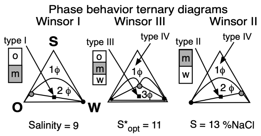
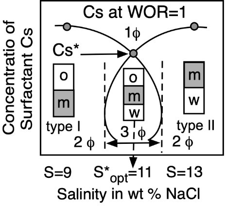
Figure 5. Top: Phase behavior at constant formulation cut for three cases of salinity (Winsor’s diagrams). Bottom: Solubilization as C_S surfactant concentration to attain a single-phase microemulsion at constant WOR = 1 cut (vertical fish diagram). In both cases the formulation scan is carried out by a change in salinity.

In the most elemental SOW ternary case containing a pure surfactant, an aqueous brine and an immiscible oil, the variables that affect physicochemical formulation were found to be the following: the surfactant characteristic features depending on at least two different aspects (i.e., its head group hydrophilicity and its tail lipophilicity), the salinity S of the water phase, and the nature of the oil, typically the alkane carbon number (ACN) for the most simple oil case, as well as the temperature and pressure.

In Winsor’s type I phase behavior, the surfactant exhibits more dominating attractive forces or interactions with water, and thus solubilizes oil in this phase micelles, with a very low concentration in the excess oil phase (essentially just above the CMC). In type II, it is the same but in the reversed way, when the surfactant has more interactions with the oil phase, thus forming inversed micelles solubilizing water inside.

In type III, the structured middle phase has an intermediate density because it contains similar amounts of oil and water. Winsor proposed for this middle phase a lamellar, more or less jellylike structure, because of some birefringence, but he mentioned that it was not necessarily a perfectly plane liquid crystal. He suggested that it might be distorted or could contain twisted lamellae with both types of micelles not necessarily spherical, nor really fully organized, but somehow linked or connected, and that it may be in a permanently changing situation. This was a very early vision from Winsor of the currently accepted bicontinuous microemulsion structure, proposed by Scriven in his excellent description [43].

Type IV is essentially a case in which there is enough surfactant (a very large concentration in practice, such as more than 20%) to cosolubilize both oil and water to produce a single phase.

In his 1954 book and final review paper [17], Winsor proposed to relate the type of SOW system with the ratio of interactions of the surfactant located at the oil and water limit. Winsor’s formulation parameter was defined according to the value of the ratio

R = Aco/Acw,     (1)

where the molecular attractive forces Aco and Acw are between the adsorbed surfactant molecule and the nearby oil (O) and water (W) molecules. R indicates the ratio of the tendency of the interface layer to become convex towards O (R > 1) or towards W (R < 1). When R = 1 the situation corresponds to an average zero curvature at the O–W limit, which could be a flat lamellar structure or complex bicontinuous arrangements of both types of swollen micelles.

It should be noted that the R ratio is only qualitative since it is not known how many oil and water molecules actually interact with a single surfactant molecule, i.e., what are the coefficients before Aco and Acw, as well as other interactions appearing in R [32],[45].

Hidrophylic Lipophilic Deviation (HLD)

The six or seven variables complex situation of a SOW was analyzed during the intensive research drive in enhanced oil recovery with surfactants in the late 1970’s [25]. A study on bi- and multidimensional scans produced an empirical relationship which was interpreted as a physicochemical correlation for the attainment of three-phase behavior, a high solubilization and a minimum interfacial tension [26] for ionic and nonionic surfactants [27,28].

The generality of the correlation for the occurrence of a so-called optimum formulation and related phenomena was expressed as the surfactant affinity difference (SAD) in 1983 [29], and its dimensionless equivalent, so-called hydrophilic-lipophilic deviation (HLD) in 2000 [30]. Conceptually, HLD is some kind of logarithmical expression of R, i.e., it is negative (respectively positive) if R < 1 (respectively R > 1). As will be more discussed later [11], HLD has the advantage of being easier to calculate because interaction energies are generally handled as summations and subtractions of chemical potential terms instead of their ratio. Hence, the so-called generalized formulation criterion, or hydrophilic-lipophilic deviation (HLD), is the difference between the numerator and denominator of R, i.e.,

HLD = Aco − Acw     (12)

By continuously changing one of the variables influencing R or HLD, through one of the interactions Aco or Acw, a so-called “formulation scan” is said to be carried out.

For instance, if the length of a surfactant alkyl tail is increased, without changing anything else, then the term Aco is going to increase, thus increasing R and HLD. If the size of a polyethoxylated surfactant head group is increased, it is now the Acw term which is increased, thus R and HLD are decreased. If the second change is carried out to exactly return to the HLD = 0 situation of three-phase behavior, then their effects are exactly compensated from the numerical point of view.

When the salinity of the aqueous phase increases, the Acw term decreases because the salt water is a less hydrophilic solvent and it thus results in a lower interaction of the aqueous phase with the surfactant head group. The Aww interaction is also decreasing, and the denominator definitively decreases, and thus R and HLD increase [32].

When the temperature is changed, most molecular interactions are altered and the discussion is not easy to handle. However, it is experimentally well known that the ionic surfactants are likely to become slightly more water-soluble when temperature increases, i.e., Acw generally increases. The opposite occurs with nonionic species whose ethoxylated part is systematically dehydrated when temperature increases, thus becoming less water-soluble. As a result, an increase in temperature tends to slightly decrease the R and HLD for ionic surfactants and to strongly increase them for nonionics.

Consequently, it may be said that along any kind of change of a formulation variable, the R or HLD criterion increases or decreases, and that at some point of the scan, a specific R = 1 or HLD = 0 value will take place. This occurrence has been called the “optimum formulation” by the people working in enhanced oil recovery, because it is where an (ultra-)low minimum interfacial tension occurs, and thus allows the crude oil displacement to happen because of the considerable modification of the capillary number [24].

At optimum formulation the partition coefficient of the surfactant between the two excess phases in a type III system is unity, which corresponds to an equal interaction of the amphiphile molecule with the oil and water or very close to its critical micelle concentrations in the excess phases. The phase behavior change produced by an increase in brine salinity is usually shown as the diagram transition WI > WIII > WII, as indicated on the top of Figure 5.

An emulsion made by stirring an equilibrated SOW system also exhibits particular characteristics at optimum formulation [13,62,63]. It inverts, as indicated by a large change in conductivity, where it passes from O/W to W/O (reference cosmetics), as the phase behavior changes from type I to type II.

The emulsion stability passes through a very deep minimum at HLD = 0, i.e., the emulsion becomes very unstable, probably because the surfactant has a lower chemical potential in the microemulsion middle phase than at the oil-water interface, where it has to be to generate stabilization mechanisms. Consequently, it may be said that at optimum formulation, the surfactant seems to be trapped in the microemulsion and that the oil/water mixture dispersed as drops by the stirring would coalesce instantly in practice, as it would be in complete absence of surfactant. This specific emulsion strong instability at optimum formulation has recently been found to match, and thus probably to result from, a very low interfacial rheology elasticity through a low dilational modulus  [64,65,66].

Additionally, emulsion viscosity is particularly low at optimum formulation, probably because the low tension favors the elongation of the drops when the emulsion is submitted to a shear. However, this viscosity minimum is not as accurate for detecting the optimum as the minimum stability.

The hydrophilic-lipophilic deviation from optimum formulation is formally similar to the empirical equation first proposed in 1979 for alkylbenzene sulfonates and other anionic and cationic surfactants likely to produce very low interfacial tension in EOR [27]. For systems containing ionic surfactants, the correlation was originally written as follows with a unit coefficient in front of the LnS term, essentially because it was the variable that was actually scanned in most experiments [27,32]. For this reason, here it will be called HLD_Lns

HLD_LnS = LnS − K_ACN ACN + σ = 0     (23)

K is the coefficient of ACN, i.e., (∂lnS/∂ACN) in the original correlations (). K was found to be 0.16 for alkylbenzene sulfonates, 0.10 for alkyl carboxylates and sulfates, 0.17 for alkyl ammonium, and 0.19 for alkyl trimethyl ammonium and alkyl pyridinium. For extended surfactants containing a polypropylene oxide intermediate group between the ionic head and the alkyl tail, K was found to depend on PON, EON, the ionic group, and the tail branching (from 0.05 to 0.14) but with no general rule found yet [76,78,79,82,85,86].

The alcohol contribution was originally indicated as an extra term called −f(A) added in Equation (2) because it is positive only for very short alcohols like ethanol or propanols and very small. For longer alcohols normally used, it is negative and linear, i.e., −f(A) = −K_A C_A, with C_A being the concentration in vol % and K_A a negative coefficient whose absolute value increases with the alcohol lipophilicity.

The following more complete correlation (3) includes the effect of temperature and pressure [87,88,89,90]. The temperature effect is small for ionic surfactant. The pressure effect reported only some time ago [90] has in most cases a very small K_p coefficient value in HLD; it is thus generally negligible at ambient conditions.

HLD_LnS = Ln(S) − K_ACN (ACN) + σ − K_AC_A − K_T (T) − K_p (P) = 0     (34)

HLD equation can be generalized so as to use it as a single expression, dividing by the coefficient of the variable which has the same meaning, i.e., K_ACN, thus becoming the “normalized” HLD_N, in which the surfactant contributing parameter SCP is also taken with a (+1) coefficient by definition.

HLD_N = SCP − (ACN − ACN_ref) + k_LnS LnS (or k_S S) − k_AC_A ± k_T (T-T_ref) − k_p (P-P_ref) = 0     (45)

In the references that are usually selected, the temperature and pressure are ambient values, i.e., T_ref = 25 °C and P_ref = 1 bar, while the salinity references are S = 0 for nonionics, or S = 1 for ionic amphiphiles (as well as S = 1 for a mixture of ionic and nonionic surfactants), and in most cases without alcohol (C_A = 0). In the current Equation (11), the oil reference could be taken as ACN_ref = 0, so that, with the previously selected references, the HLD_N = 0 equation can be simply be written as SCP = (P)CAN.

Relation of HLD Values with Micro-, Mini-, and Macroemulsion Properties

Emulsion persistence has been systematically studied in many reports describing the numerous phenomena involved [127,128,129]. No matter the ordinate stability scale, it happens that very close to optimum formulation, in the narrow HLD_N interval from −5 to +5, the emulsions are very unstable. The handling of HLD by changing one or two variables enables the emulsion manufacturer to be exactly in the desired stability or instability zone. This is why manipulating the HLD is an extremely useful technique for the practical use of formulation. At optimum formulation SOW systems exhibits not only a very strong instability, but it also indicates that, at some distance from HLD_N = 0, i.e., in the 10–20 unit range on both sides, there is a stable zone for the two types of emulsions.

The formulation-composition diagram

The formulation-composition (WOR, Water-Oil Ratio) diagram depicted in Figure 16, is an important tool for understanding the changes that occur in SOW when variables are changed. The emulsion inversion is a horizontal line at HLD_N ~ 0 with the WIII phase behavior in the WOR central part. In this range, the HLD is the unique criterion to attain O/W or W/O types so-called A+ and A- “normal” emulsions, in which the continuous phase is the one containing most of the surfactant. In the extreme WOR zones, called B and C, the normal emulsions occur when the HLD matches the occurrence of the continuous phase with most of the surfactant, i.e., B+ (respectively C-), which may be considered as the continuity of the A+ (respectively A-) zone with a high dilution, i.e., a large excess of the external phase.

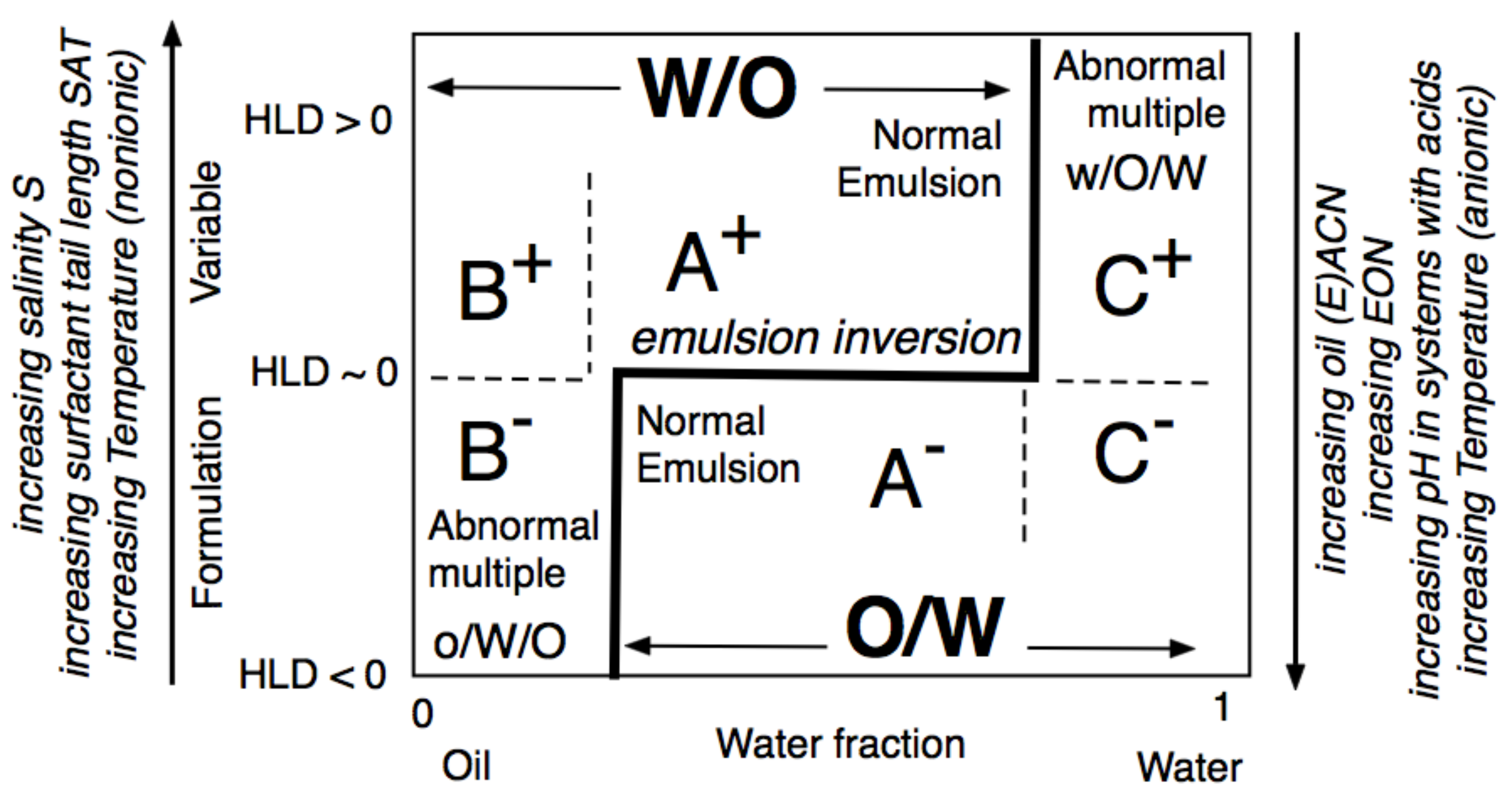
Figure 16. Classical formulation-composition diagram (HLD-WOR) showing the inversion line and emulsion types.

On the contrary, the B– and C+ zones are said to be “abnormal” because most of the surfactant is not in the emulsion external phase. This is the reason why these zones are exhibiting “multiple” emulsions in some places, with droplets in drops forming the “internal” emulsion, and drops in a continuous phase forming the “external” one, i.e., o/W/O in B– and w/O/W in C+, with the low case letter indicating the phase of the smaller droplets inside the drops. The formation of multiple emulsion is due to a conflict between the formulation and the composition, and it depends on the way the emulsification process is carried out, in particular, it can be made in different steps or produced spontaneously [152,153,154,155].

The two lateral branches of the inversion line, depicted in Figure 17 are mostly vertical, are due to the presence of different mechanisms which are independent from HLD. This type of inversion thus mainly depends on the WOR, with a strong tendency to have the one with the larger proportion as an external phase. This is why the inversion vertical line is on the right or the left side, depending on the HLD favoring a curvature matching a W/O or O/W emulsion. The vertical line position was also found to depend on other conditions which do not appear on this map, such as the mixing apparatus features that can influence the local WOR in the mixed zone, as well as the stirring energy and the intensity of shearing, and the relative viscosity of the phases. This inversion which is so-called “catastrophic” because of its characteristics, is not necessarily the same in the two directions of change, i.e., when adding oil or adding water, and it can involve a hysteresis that tends to increase when the formulation deviates from HLD = 0. This hysteresis means that dynamic changes in WOR (i.e., adding water or adding oil when stirring) can produce delays, or somehow push the inversion occurrence, thus displacing its position. As a consequence, these vertical parts on the inversion line can be slanted in one direction or the other depending on the direction of WOR change.

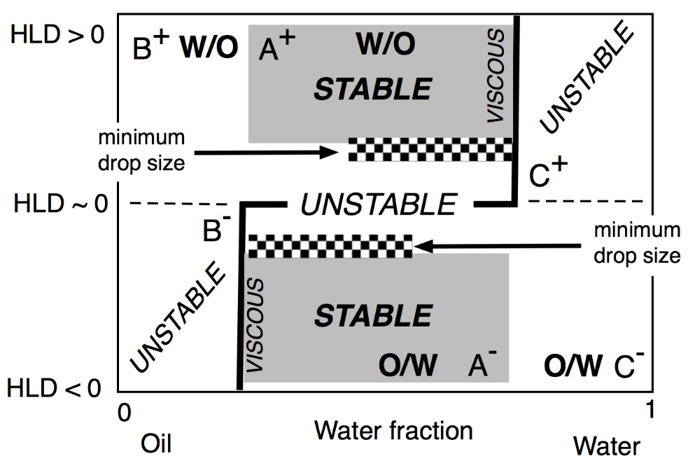
Figure 17. Classical formulation-composition diagram (HLD-WOR) showing the basic properties (stability, drop size and viscosity) as described a long time ago [155].

In any case, this change in property from place to place in this kind of map indicates that dynamic processes are often a means to benefit from several favorable properties in a path on the map with a number of subsequent steps, often with a horizontal, vertical or slanted crossing of the inversion line [149,159,160,161,162,163,164].

The complex case of SOW non-linear mixtures

There are instances where the very straightforward case of HLD_N linear relationship isn't apparent. These happen due to the occurrence of non-linear effects in mixtures of the components that are present in SOW systems. Some specific cases can be mentioned, particularly the effect of non-linearity in complex oil, salt or surfactant mixtures.

Equivalent Alquil Chain Number (EACN)

When the oil phase contains various substances, a linear mixing rule is generally valid if the species involved are not very different, in particular in their structure and polarity. For instance, a hexane-hexadecane mixture perfectly follows a linear equation with the number of carbon atoms in the oil as can be seen in the next equation, where the X_i is the fraction (molar in theory but often simply volumetric) of the “i” specie in the mixture.

EACN_MIX = ∑ X_i EACN_i     (56)

Oils of diverse nature generate non-linear mixture rules. For example, when benzene is added to the tetradecane, the LnS* decreases very quickly, certainly because the benzene tends to accumulate close to the interface, and results in a strong change [113,176]. However, on the other side, when some tetradecane is added to benzene, the oil LnS* practically does not change because the tetradecane does not go close to the interface, where the benzene occupies almost all the volume.

Equivalent Salinity

In many cases, the aqueous phase contains different salts, in particular in a petroleum reservoir, in wastewater, and in blood. The HLD linear variation with salinity as LnS seems to be general for ionic surfactant systems, even if the concentration is not expressed in wt% but in mol/liter, i.e., with another scale, which only changes the salinity term coefficient in the HLD_N expression.

The variation of the negative counter-ion (for instance a change from sodium chloride to sodium sulfate or phosphate) can be taken into account with an equivalence coefficient 2/(1 + Z), where Z is the valency of the anions [75]. This term enters the constant in the HLD_N equation and the equivalence is easy to handle.

However, this is not the case for the variation of the cation (for instance from sodium to calcium or aluminum chloride) and a general salinity equivalence is not available yet, although some trends have been proposed [103,126,184].

Equivalent SCP in Surfactant Mixtures

The use of surfactant mixtures is a very important subject, first because, in many systems, the S, (E)ACN, T and P values are fixed by the application. A required SCP value can thus be calculated to produce HLD = 0 in order to attain optimum formulation or a different goal, for instance, HLD_N ~ −6 or −8 to produce an O/W small-drop nanoemulsion.

Since it is highly unlikely that a commercial product has the proper SCP to exactly attain the goal, a mixture of at least two surfactants is required. Back in 1979, the basic mixing rules were studied at the same time as the SAD/HLD concept for the EOR application [69]. These results were written as follows when the optimum was detected by a salinity scan for two or more similar ionic surfactants:

LnS_MIX = X₁ LnS₁ + X₂ LnS₂ or LnS_MIX = ∑ X_i LnS_i     (67)

Or with EON scans for ethoxylated nonionics where ∂β/∂ACN = −∂EON/∂AC N slope K = −0.15

EON_MIX = X₁ EON₁ + X₂ EON₂ or EON_MIX = ∑ X_i EON_i     (78)

This is equivalent to HLD_MIX = ∑ X_i HLD_i only if the K coefficient is the same for all the surfactants used, which is not always true in particular in a mixture of ionics with different Ks in front of ACN, and for ionic/nonionic mixtures where the definitions of K are different. To avoid this problem, it is absolutely necessary to use the normalized HLD_N for such mixtures, and thus the surfactant contribution parameter SCP with the same coefficient as the real or virtual scan variable, i.e., SCP = N_MIN, σ/K, β/K, Cc/K, PIT/K in the first generation of equations.

Final remarks

Using a sound knowledge of physicochemical formulation, HLD_N parameter, a general HLD-WOR map, and carrying out a few experiments to generate the corresponding know-how, makes it possible to conduct a few effective trials to obtain an original solution for very complex SOW systems. Now, the possibilities are very numerous because the exact position of the frontiers also depends on some specificities of the surfactant(s), oil(s), and brine, as well as cosurfactants, and polymers.

This means that each research and development center which prepares an emulsion with a specific application needs to improve its understanding and build up appropriate know-how for its business. This is generally a matter of getting some practical training from a university working with the industrial sector. Then the research and development professionals have to start working on that, trial after trial, in equilibrated and dynamic processes, and, after 10 years of accumulated experience, they will be able to provide an optimized solution in a few days only.