Your browser does not fully support modern features. Please upgrade for a smoother experience.
Please note this is a comparison between Version 1 by Xiaohan Wang and Version 3 by Xiaohan Wang.
Proso millet (Panicum miliaceum L.) or broomcorn millet is among the most important food crops to be domesticated by humans; it is widely distributed in America, Europe, and Asia.
- gene migration
- population structure
- genetic diversity
- association analysis
- SSR marker
- total phenolic content
1. Introduction
Proso millet (Panicum miliaceum L.) is an annual monocotyledonous grass crop. Archaeological evidence indicates that this crop was first domesticated in northern China about 10,000 years ago [1]. Today, proso millet is widely distributed in the Americas, Europe, and Asia, and is still among the most important food crops worldwide [2]. Proso millet has a short growth cycle and low water requirement; rotation with proso millet can maintain moisture in deep soil layers, control winter weeds, and reduce the occurrence of pests and diseases, making it an ideal rotation crop for winter wheat [3]. When other crops fail to harvest or planting is delayed due to adverse weather, proso millet can be planted as an intercropping crop to reduce economic losses [4]. Proso millet is also widely used in the bird, pet feed, snack food, and wine-making industries [5]. At present, the demand for proso millet is highest for bird feed production [6].
Many previous studies have examined the genetic diversity of proso millet, including in China (using 88 accession core collections selected from 8,515 materials based on 67 proso millet-specific single-sequence repeat (SSR) markers) [5], and Canada and the USA (using 12 accessions based on amplified fragment length polymorphisms [AFLPs]) [7], as well as in six countries using 50 accessions based on 25 SSR markers [8], and 25 countries using 90 accessions based on 100 SSR markers [6]. However, these studies focused on explaining the genetic diversity and clades of local proso millet populations.
The evolutionary origin of proso millet has always been controversial, with domestication centers being proposed in multiple regions of China and Eastern Europe [9], and in a single center in China [10]. Accumulating evidence from archaeological, diversity and phylogenetic studies, among others, suggests that that proso millet originated from carbonized grains about 10,000 years ago; these grains were unearthed at the Cishan site in China [1]. The Dadiwan site in the Loess Plateau, and the Xinglonggou site in Inner Mongolia, have also yielded carbonized proso millet particles believed to be about 8000 years old [11][12][11,12]. Another study suggested that the European proso millet first appeared about 7000 years ago [13]. This was revised to 3600 years ago based on direct measurement of the crop remains [14]. However, it is difficult to determine the place of origin of proso millet based on the distribution of its wild ancestors, because this species is easily back-mutated from domesticated crops to weeds [13]. A study using SSR markers to genotype domesticated proso millet in China concluded that genetic diversity in China was highest on the Loess Plateau [10]. One study used 98 accessions from Eurasia and 16 SSR markers to explore the possibility that Eastern Europe is one of several sites of origin of domesticated proso millet [9]. However, due to the limited availability of accessions, comprehensive analysis of genetic diversity is difficult and observer bias can affect diversity analysis.
Several studies have reported benefits of proso millet polyphenols, such as anti-inflammatory effects [15], anti-proliferative effects in colorectal cancer [16], liver protection due to syringic acid [17], free radical scavenging by ferulic acid, and antioxidant activity [18]. Proso millet varieties differ in terms of free syringic acid, ferulic acid, chlorogenic acid, caffeic acid, and p-coumaric acid content [19]. Total phenolic content (TPC) mainly depends on the variety, rather than type or color, of proso millet, although TPC and antioxidant capacity are also significantly affected by climatic and environmental conditions [20].
Breeders use genetic markers to assess the phenotypes of target traits in the early stages of the growth cycle; this approach greatly shortens the research cycle and reduces the workload associated with crop breeding. Molecular markers are essential for improving traits that cannot be directly measured. The development of molecular markers for phenols has allowed rapid estimation of the types and quantity of phenolic compounds in individual plants. however, no studies have developed molecular markers of TPC and antioxidants in proso millet, although such markers have been developed for other plant taxa. For example, molecular markers were developed to identify phenolic compounds in wild and cultivated barley [21], and a genome-wide association study identified 11 quantitative traits related to nucleosides in snap bean [22]. Genome-wide association studies have revealed that apple polyphenols are controlled by 4-O-caffeoylquinic acid and procyanidins B1, B2, and C1, and demonstrated the applicability of these markers to marker-assisted breeding. Although polyphenols are important components of the human diet, breeders have not widely regarded them as breeding targets; however, polyphenolic enhancement of nutritional properties may become a future breeding trend. With the improvement of the cultivation environment and the impact of cash crops, locally endemic varieties of proso millet are rapidly disappearing, which greatly affects the diversity of proso millet populations. Therefore, as genetic important resources, proso millet and other small grain crops have been a focus of research.
2. Genetic Diversity Analysis
In a preliminary experiment, proso millet samples were amplified; there were 481 expressed sequence tag (EST) SSR markers, 37 EST-SSR markers that can be successfully amplified in the DNA of all individuals and have polymorphisms were screened out (Supplementary Dataset 1). Among 578 proso millet accessions collected in 17 countries of origin, 37 pairs of SSR primers were used to amplify 151 alleles (Supplementary Dataset 2).
Genetic diversity analysis showed that, among the 578 germplasms, the number of alleles (Na) per locus ranged from 2 to 7, with an average of 4.0811. The number of amplified genotypes (Ng) ranged from 2 to 17, with an average of 4.7838. Shannon’s information index (I) ranged from 0.0803 to 1.436, with an average of 0.387. Observed heterozygosity (Ho) ranged from 0 to 0.0657, with an average of 0.0032, indicating gene flow among individuals and genotypes. The genetic diversity value (H) ranged from 0.0274 (SSR-143) to 0.7331 (SSR-365), with an average of 0.19. The fixation index (Fst) is used to measure the proso millet population genetic differentiation. Among the 37 SSR markers, each marker provided a different ability to distinguish genetic differentiation, ranging from 0.0452 (SSR-458) to 0.6783 (SSR-128), with an average of 0.4545. The polymorphic information content (PIC) value of the SSRs ranged from 0.0273 (SSR-143) to 0.6884 (SSR-365), with an average of 0.1735. The average major allele frequency (MAF) was 0.8740, with a range of 0.3789 (SSR-365) to 0.9862 (SSR-143). Three SSRs showed high PIC values, SSR-203 (0.5086), SSR-232 (0.5944), and SSR-365 (0.6884), i.e., values exceeding the critical value of 0.5. The detailed parameters are listed in Table 1 and the genetic diversity analysis results for each place of origin are listed in Table 2. Genetic resources from Ukraine showed the highest diversity index (0.247 ± 0.247), followed by Russia (0.215 ± 0.183) and South Korea (0.156 ± 0.192).
Table 1. Diversity information provided by 37 single-sequence repeat (SSR) markers.
| Locus | Ng a | Na b | I c | Ho d | H e | Fst f | PIC g | MAF | RUS | THA | TJK | TUR | UKR | UZB | |
|---|---|---|---|---|---|---|---|---|---|---|---|---|---|---|---|
| BOL | 0.078 *** | - |
4. Discussion
4.1. Gene Flow and Geographic Distributions
The gene flow analysis results did not identify a single domestication center for proso millet, as cluster 4 did not clearly originate from cluster 5. Our results could reflect either single or multiple domestication centers, as population structural analysis cannot assume that K = 1 [9]. Our gene flow analysis results were insufficient to demonstrate that cluster 4 originated from cluster 5; they only showed that gene flow from cluster 5 to cluster 4 was greater than that from cluster 4 to cluster 5. According to the local diversity of each cluster (Table S1) and the gene flow analysis results, we determined the primary or secondary center of origin of each clusters. Nepal (and its surrounding areas) was the secondary center of origin for cluster 6. Our phylogenetic, population structure, and gene flow analysis results indicated that cluster 6 originated from cluster 5, and that the secondary center of origin was in Nepal and its surrounding areas, in high-latitude and high-altitude areas. This is similar to the three gene microcenters detected in Turkey, where the cultivation environment was exceptionally well-suited to wheat domestication [24]. In South Korea, cluster 1 was found to have derived from cluster 5, which is a unique germplasm resource. A previous study also identified Japan as an origin point for proso millet cluster 1 [9].
Cluster 1 is considered to be a unique proso millet germplasm resource that was domesticated in South Korea. Although one germplasm resource was collected in Russia, and one in Thailand, while two germplasms were collected in India, gene flow analysis showed that they were all derived from the Korean germplasm. Cluster 2 is distributed only in Asia. Gene flow analysis showed that these two clusters were introduced from China to South Korea, Mongolia, Uzbekistan, and India, and then from India to Russia and Thailand. Cluster 3 is widely distributed in Eurasia, with a diversity index of 0.143174. However, our gene flow results showed that cluster 3 originated in the fertile crescent of Turkey and then spread to France and India, from which it subsequently spread to Central Asia (Uzbekistan and Turkey) and finally to East Asia. In cluster 4, the highest genetic diversity was detected in germplasms native to Turkey; however, gene flow analysis showed that Turkey’s seed resources migrated from China to Uzbekistan, and then to Turkey. Cluster 4 originated in China and was introduced via Mongolia to Russia and North Korea. Germplasms of China and Mongolia also spread to Uzbekistan, and then from Uzbekistan to India, India to Thailand, Uzbekistan to Turkey, and Turkey to Ukraine. Cluster 5 occurred frequently in East, Southeast, and South Asia, and evolved according to a network pattern. Cluster 5 had the highest diversity; gene flow analysis pointed to China as the center of domestication, from which it migrated to Europe (Ukraine) via different routes, and then to Mongolia and finally back to China. Cluster 6 showed high abundance in high-latitude and high-altitude regions; it originated in Nepal and was then introduced into Ukraine, Russia, and Mongolia, and then into South Korea from Ukraine.
By combining the phylogeny, diversity, population structure, M, and gene flow analysis results, we obtained expansion paths for each cluster of proso millet that were consistent with a previously established archaeological map of the agricultural origins and migration of Neolithic and formative cultures [25]. In this study, we provided SSR markers combination of each cluster to identify the cluster where an individual is located (Table S2). The highest diversity was found in clusters 4 and 5, and the longest branches (indicating the longest genetic distance from other germplasms) were found in clusters 3 and 5. Regions with high diversity were not identified as regions of origin, likely because gene introgression from other proso millet clusters resulted in high diversity. In a future study, we will amplify and sequence these genotypes to identify the markers with the greatest diversity (SSR-203, SSR-232, or SSR-365) as plant DNA barcodes, to detect other known antioxidants. Then, we will use these markers to accurately determine genotype composition and compare it with a neutral model to shed light on the population expansion associated with bottleneck events.
In this study, the population genetic diversity is low, and the genetic differentiation is high. We believe that the reason is that the proso millet is an inbred plant. Self-crossing reduces the effective population size and effective recombination rate. Compared with outcrossing, it directly leads to a decrease in polymorphism and an increase in linkage disequilibrium [26]. The increase in isolation between populations also directly stems from selfing or indirectly from evolutionary changes, leading to greater differentiation of molecular markers than during outcrossing. The lower effective recombination rate increases the possibility of free-riding and further reduces the internal diversity of inbreds, thereby increasing their genetic differentiation [27].
In addition, in the process of agronomic traits data collation, we observed that the standard deviation within each sub-cluster was very high (Table 4). The degradation of cultivars of proso millet to wild species may be the main reason for the large standard deviation. In this study, the population of 578 accessions is composed of wild species and landraces. Landraces degenerate into wild species, some genotypes are preserved, and may still be clustered with local landraces, but agronomic traits show differences. Feral derivatives of crop varieties may show a similar phenotype to that of the crop ancestor [28].
Table 4. Differences in agronomic traits within each subcluster branch.
| No | Cluster | Sub-Cluster | NB/P a |
|---|---|---|---|
| 0.1705 | |||
| 0.1561 | |||
a Number of genotypes in which each locus amplified alleles; b observed number of alleles; c Shannon’s information index; d observed heterozygosity; e Nei’s (1973) gene diversity; f F-statistic value for evaluation of geographical differentiation; g polymorphism information content; and h major allele frequency.
Table 2. Genetic diversity information of each origin accession.
| Origin | Ng a | Na b | I c | Ho d | HD bH e | PIC f | HT MAF gh |
|---|---|---|---|---|---|---|---|
| c | |||||||
| SSR-31 | 3 | 3 | 0.83 | 0 | 0.5185 | 0.5083 | |
| South Korea | 3.919 ± 1.402 | 3.73 ± 1.223 | 0.312 ± 0.338 | 0.002 ± 0.006 | 0.156 ± 0.192 | 0.145 ± 0.156 | 0.892 ± 0.154 |
Pairwise Fst is used to evaluate the degree of genetic differentiation among 17 countries of origin (Table 3). Pairwise comparisons between accessions from different origins showed that the Fst values ranged from 0.027 between Czechoslovakia (CSK) and Kazakhstan (KAZ) to 0.2699 between Turkey (TUR) and France (FRA). The lowest differentiation was observed between the population composed of germplasm originating from Korea and 17 other populations, 3 and 14 of which showed low (Fst = 0.05) and moderate (Fst = 0.15) differentiation. The degree of differentiation among the Russian (RUS), Ukrainian (UKR), and Chinese (CHN) groups was lower than among other groups. A comparison of populations native to China with other populations showed that 14 populations had a moderate degree of differentiation, whereas 3 had a high degree of differentiation (Fst = 0.15–0.25): Bolivia (BOL), FRA, and Tajikistan (TJK). The TUR population showed the highest degree of differentiation from FRA (Fst = 0.2699), followed by the Iranian (IRN), North Korean (PRK), and South Korean (KOR), and CHN (Fst = 0.1) populations. TUR, TJK, BOL, CSK, and Azerbaijan (AZE) showed the greatest within-country differentiation among populations. The results of the global Fst for all populations show that UZB, IND, RUS, IRN, and CSK are all low genetically differentiated. The populations of KAZ, FRA, PRK, MNG, and TJK show a moderate degree of genetic differentiation. The populations of CHN, BOL, THA, KOR, NPL, TUR, AZE and UKR show high genetic differentiation.
Table 3. Differentiation among origin populations according to the fixation index (Fst).
| AZE | BOL | CHN | CSK | FRA | IND | IRN | PL KAZ | KOR | d | PW MNG | NPL | e | SD fPRK | PH g | ||||||||||||
|---|---|---|---|---|---|---|---|---|---|---|---|---|---|---|---|---|---|---|---|---|---|---|---|---|---|---|
| 0.4277 | 0.5952 | |||||||||||||||||||||||||
| 1 | A | A1 | 8.74 ± 1.98 | 31.99 ± 3.95 | 93.84 ± 5.84 | 29.81 ± 3.91 | 8.34 ± 1.9 | 2.75 ± 0.39 | 106.55 ± 14.2 | SSR-67 | 5 | 5 | ||||||||||||||
| North Korea | 1.486 ± 0.683 | 1.486 ± 0.683 | 0.3864 | 0 | 0.1568 | 0.077 ± 0.231 | 0 ± 00.5596 | 0.1527 | 0.917 | |||||||||||||||||
| CHN | 0.133 *** | 0.16 *** | - | 0.051 ± 0.149 | 0.148 ± 0.201 | 0.858 ± 0.197 | ||||||||||||||||||||
| 1 | A2 | 7.73 ± 1.94 | 27.13 ± 5.6 | 92.56 ± 6.71 | 25.73 ± 7.56 | 7.3 ± 3.34 | 2.23 ± 0.67 | 84.02 ± 31.64 | SSR-70 | 4 | 4 | 0.269 | 0 | 0.1208 | 0.211 | 0.1154 | 0.936 | |||||||||
| CSK | 0.189 *** | 0.232 *** | 0.104 *** | - | ||||||||||||||||||||||
| 2 | B | B1 | 7.58 ± 2.15 | 23.34 ± 5.23 | 93.34 ± 5.32 | 19 ± 6.37 | 5.14 ± 2.65 | SSR-71 | 3 | 3 | 0.1518 | 0 | 0.0575 | 0.1335 | 0.0566 | 0.9706 | ||||||||||
| FRA | 0.081 *** | 0.124 *** | 0.156 *** | 0.162 *** | - | |||||||||||||||||||||
| 26.45 ± 6.02 | 7.93 ± 3.18 | 2.43 ± 0.57 | 92.78 ± 27.58 | SSR-82 | 6 | 6 | 0.4553 | 0 | 0.1926 | 0.4387 | 0.1857 | 0.8962 | ||||||||||||||
| IND | 0.093 *** | 0.114 *** | 0.071 *** | 0.115 *** | 0.096 *** | - | SSR-85 | 3 | 3 | |||||||||||||||||
| IRN | 0.133 *** | 0.1527 | 0 | 0.0606 | 0.0957 | 0.179 *** | 0.065 *** | 0.098 *** | 0.191 *** | 0.087 ***0.0593 | -0.9689 | |||||||||||||||
| SSR-86 | ||||||||||||||||||||||||||
| 3 | 2 | 2 | 0.1387 | 0 | 0.0603 | 0.119 | 0.0585 | 0.9689 | ||||||||||||||||||
| SSR-92 | 3 | 3 | 0.5072 | 0 | 0.2864 | 0.118 *** | 0.04 *** | 0.08 *** | 0.134 *** | 0.159 *** | - | |||||||||||||||
| 1.68 ± 0.63 | 54.76 ± 28.67 | |||||||||||||||||||||||||
| 2 | B2 | 8.16 ± 2.13 | 29.83 ± 5.27 | 94.78 ± 5.19 | C | C1 | 8.1 ± 2.04 | 29.39 ± 5.93 | 94.09 ± 5.94 | 26.78 ± 7.28 | 7.1 ± 2.64 | 2.37 ± 0.68 | 89.06 ± 30.08 | |||||||||||||
| 3 | KAZ | 0.162 *** | 0.205 *** | 0.089 *** | 0.027 *** | 0.135 *** | 0.092 *** | 0.098 *** | - | 0.6762 | 0.2534 | 0.8304 | ||||||||||||||
| KOR | 0.127 *** | 0.143 *** | 0.055 *** | 0.114 *** | 0.13 *** | 0.038 *** | 0.081 *** | 0.089 *** | - | SSR-100 | 4 | 4 | ||||||||||||||
| MNG | 0.135 *** | 0.313 | 0 | 0.1341 | 0.0523 | 0.145 *** | 0.088 *** | 0.136 *** | 0.132 *** | 0.063 ***0.1294 | 0.127 ***0.9291 | |||||||||||||||
| 0.109 *** | 0.041 *** | - | SSR-109 | 3 | 3 | 0.2646 | 0 | 0.1237 | ||||||||||||||||||
| NPL | 0.1991 | 0.1175 | 0.9343 | |||||||||||||||||||||||
| 0.165 *** | 0.186 *** | 0.121 *** | 0.117 *** | 0.145 *** | 0.082 *** | 0.126 *** | 0.09 *** | 0.065 *** | 0.078 *** | - | SSR-120 | 5 | 5 | 0.6157 | 0 | 0.2895 | 0.4262 | 0.2723 | 0.8356 | |||||||
| SSR-121 | 2 | 2 | 0.0803 | 0 | 0.0307 | 0.0705 | 0.0302 | 0.9844 | ||||||||||||||||||
| SSR-127 | 3 | 3 | 0.1354 | 0 | 0.0508 | 0.0765 | 0.05 | 0.974 | ||||||||||||||||||
| SSR-128 | 3 | 3 | 0.3346 | 0 | 0.1809 | 0.6783 | 0.1651 | 0.8997 | ||||||||||||||||||
| SSR-129 | 3 | 3 | 0.2078 | 0 | 0.0837 | 0.0707 | 0.0819 | 0.9567 | ||||||||||||||||||
| SSR-131 | 5 | 5 | 0.1612 | 0 | 0.0544 | 0.1865 | 0.05390.5086 | |||||||||||||||||||
| China | 3.108 ± 0.98 | 3.054 ± 0.928 | 0.188 ± 0.298 | 0.004 ± 0.013 | 0.333 ± 0.147 | 0.299 ± 0.13 | 0.545 | |||||||||||||||||||
| 0.857 ± 0.151 | ||||||||||||||||||||||||||
| Mongolia | 2.324 ± 1.275 | 2.27 ± 1.106 | 0.248 ± 0.254 | 0.005 ± 0.018 | 0.13 ± 0.14 | 0.151 ± 0.175 | 0.893 ± 0.155 | |||||||||||||||||||
| Uzbekistan | 1.243 ± 0.488 | 1.243 ± 0.488 | 0.068 ± 0.196 | 0.007 ± 0.041 | 0.047 ± 0.137 | 0.079 ± 0.153 | 0.912 ± 0.176 | |||||||||||||||||||
| Thailand | 1.541 ± 0.682 | 1.541 ± 0.682 | 0.142 ± 0.338 | 0.003 ± 0.016 | 0.081 ± 0.191 | 0.103 ± 0.134 | 0.92 ± 0.124 | |||||||||||||||||||
| India | 1.973 ± 1.174 | 1.919 ± 1.075 | 0.198 ± 0.338 | 0.002 ± 0.008 | 0.099 ± 0.18 | 0.094 ± 0.138 | 0.932 ± 0.116 | |||||||||||||||||||
| Nepal | 1.27 ± 0.684 | 1.243 ± 0.633 | 0.174 ± 0.353 | 0.007 ± 0.044 | 0.097 ± 0.196 | 0.044 ± 0.112 | 0.969 ± 0.079 | |||||||||||||||||||
| Turkey | 2.811 ± 1.135 | 2.811 ± 1.135 | 0.375 ± 0.409 | 0.004 ± 0.013 | 0.198 ± 0.225 | 0.255 ± 0.176 | 0.817 ± 0.146 | |||||||||||||||||||
| Russia | 2.892 ± 2.576 | 2.568 ± 1.516 | 0.417 ± 0.324 | 0.008 ± 0.031 | 0.215 ± 0.183 | 0.131 ± 0.193 | 0.892 ± 0.185 | |||||||||||||||||||
| Ukraine | 2 ± 1.115 | 1.973 ± 1.078 | 0.42 ± 0.436 | 0.01 ± 0.045 | 0.247 ± 0.247 | 0.198 ± 0.191 | ||||||||||||||||||||
| PRK | 0.162 *** | 0.206 *** | 0.07 *** | 0.096 *** | 0.189 *** | 0.11 *** | 0.848 ± 0.164 | 0.079 *** | 0.086 *** | 0.088 *** | 0.126 *** | 0.134 *** | - | |||||||||||||
| RUS | 0.085 *** | 0.094 *** | 0.07 *** | 0.128 *** | 0.096 *** | 0.025 *** | 0.103 *** | 0.104 *** | 0.031 *** | 0.032 *** | 0.073 *** | 0.109 *** | - | |||||||||||||
| THA | 0.116 *** | 0.122 *** | 0.096 *** | 0.125 *** | 0.114 *** | 0.045 *** | 0.12 *** | 0.098 *** | 0.057 *** | 0.063 *** | 0.099 *** | 0.111 *** | 0.052 *** | - | ||||||||||||
| TJK | 0.054 *** | 0.105 *** | 0.15 *** | 0.216 *** | 0.108 *** | 0.121 *** | 0.16 *** | 0.189 *** | 0.15 *** | 0.158 *** | 0.17 *** | 0.198 *** | 0.107 *** | 0.158 *** | - | |||||||||||
| TUR | 0.208 *** | 0.248 *** | 0.1 *** | 0.215 ** | 0.27 *** | 0.172 *** | 0.114 *** | 0.226 *** | 0.145 *** | 0.181 *** | 0.225 *** | 0.133 *** | 0.17 *** | 0.9723 | ||||||||||||
| 0.207 *** | 0.238 *** | - | SSR-142 | 3 | 3 | 0.1067 | ||||||||||||||||||||
| UKR | 0.111 *** | 0.146 *** | 0.074 *** | 0.143 *** | 0.133 *** | 0.067 *** | 0.124 *** | 0.118 *** | 0.054 *** | 0.047 *** | 0.09 *** | 0 | 0.0375 | 0.1257 | 0.0371 | 0.981 | ||||||||||
| UZB | 0.06 *** | 0.051 *** | 0.11 *** | 0.174 *** | 0.13 *** | 0.088 *** | 0.116 *** | 0.147 *** | 0.094 *** | 0.096 *** | 0.117 *** | 0.133 *** | 0.06 *** | 0.104 *** | 0.097 *** | 0.181 *** | 0.102 *** | - | SSR-143 | 5 | 5 | 0.0898 | ||||
| Pop18 | 0.341 *** | 0.272 *** | 0 | 0.0274 | 0.0521 | 0.0273 | 0.9862 | |||||||||||||||||||
| 0.253 *** | 0.137 ** | 0.212 *** | 0.111 ** | 0.131 *** | 0.157 *** | 0.313 *** | 0.221 *** | 0.313 *** | 0.215 *** | 0.119 | 0.307 *** | 0.237 *** | 0.324 *** | 0.431 *** | 0.101 *** | SSR-144 | 8 | 7 | 0.3365 | 0.0017 | 0.1199 | 0.5294 | 0.12 | 0.9369 | ||
| SSR-146 | 4 | 4 | 0.0948 | 0 | 0.0308 | 0.0724 | 0.0306 | 0.9844 | ||||||||||||||||||
| SSR-182 | 3 | 3 | 0.2275 | 0 | 0.0934 | 0.0609 | 0.0912 | 0.9516 | ||||||||||||||||||
| SSR-195 | 3 | 3 | 0.5953 | 0 | 0.3512 | 0.6687 | 0.3024 | 0.7803 | ||||||||||||||||||
| SSR-203 | 8 | 7 | 1.0966 | 0.0017 | 0.5816 | 0.4101 | SSR-232 | 17 | 6 | 1.2808 | 0.0657 | 0.6305 | 0.5055 | 0.5944 | 0.5536 | |||||||||||
| SSR-331 | 4 | 4 | 0.5478 | 0 | 0.2672 | 0.4275 | 0.2511 | 0.8495 | ||||||||||||||||||
| SSR-357 | 8 | 5 | 0.3716 | 0.0052 | 0.1535 | 0.3719 | 0.1491 | 0.9187 | ||||||||||||||||||
| SSR-365 | 7 | 7 | 1.436 | 0 | 0.7331 | 0.4282 | 0.6884 | 0.3789 | ||||||||||||||||||
| SSR-384 | 10 | 6 | 0.5456 | 0.0104 | 0.2291 | 0.2318 | 0.2178 | 0.878 | ||||||||||||||||||
| SSR-386 | 6 | 6 | 0.1698 | 0.0035 | 0.0641 | 0.0604 | 0.0648 | 0.9663 | ||||||||||||||||||
| SSR-394 | 4 | 4 | 0.7938 | 0.0017 | 0.52 | 0.5587 | 0.4107 | 0.5433 | ||||||||||||||||||
| SSR-404 | 5 | 4 | 0.1716 | 0.0017 | 0.0672 | 0.3127 | 0.0642 | 0.9663 | ||||||||||||||||||
| SSR-409 | 4 | 3 | 0.1446 | 0.0104 | 0.0636 | 0.0642 | 0.062 | 0.9671 | ||||||||||||||||||
| SSR-420 | 4 | 3 | 0.0873 | 0.0087 | 0.034 | 0.0575 | 0.0287 | 0.9853 | ||||||||||||||||||
| SSR-430 | 4 | 4 | 0.8734 | 0 | 0.4998 | 0.3517 | 0.44 | 0.6574 | ||||||||||||||||||
| SSR-448 | 3 | 3 | 0.0885 | 0 | 0.0307 | 0.047 | 0.0304 |
** p < 0.01; *** p < 0.001. Fst value is 0-0.05, the degree of genetic differentiation among populations is low; Between 0.05–0.15, there is a moderate degree of genetic differentiation among populations; Between 0.15–0.25, the degree of genetic differentiation among populations is high; Above 0.25, there is great genetic differentiation among populations.
3. Population Structure and Phylogenetic Analysis
We performed population structural analysis using the Structure Harvester program [23], with the number of subpopulations (K) ranging from 2 to 20. The results showed that ΔK reached a maximum (16.65391) at K = 3, indicating that this was the most suitable K (Figure 1a), followed by 10 (ΔK = 11.57047), 8 (5.402586), and 6 (3.059784). The 578 accessions from various regions were therefore classified into three subgroups (Figure 1b). Individuals of the three subgroups were widely distributed in Eurasia (Figure 1c), of which subpopulations B (orange) and C (azure) were distributed in Eurasia, and subpopulations A (dark blue) in Asia.
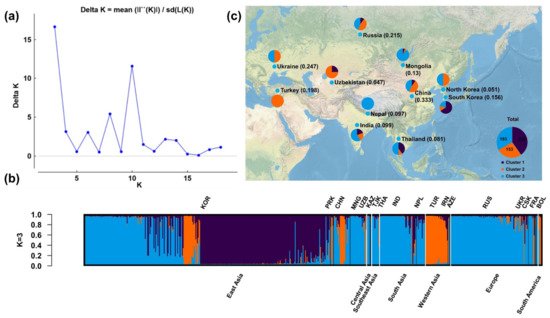
Figure 1. Population structural analysis results. (a) Determination of the optimal number of subpopulations (K) according to the values of ΔK calculated by the Structural Harvester program. (b) Corresponding population structure diagram and (c) geographical distribution for K = 3.
Phylogenetic analysis resulted in three clusters (Figure 2); individuals located within these clusters were consistent with those grouped by population structure analysis. We used XLSTAT software v2019 (Addinsoft, Paris, France) to test the significance of the geographic distribution of 3 clusterings of proso millet through the chi-square test, and verify the results of the chi-square test with Fisher’s exact test. The results of the chi-square test showed that the overall p-value was <0.0001, which was lower than the significance level of 0.05. Therefore, we reject the null hypothesis that cluster and geographic distribution are independent, and the risk of error is less than 0.0001. Fisher’s exact test results that 17 of the 18 p-values are lower than the significance level 0.05. Fisher’s exact test also leads to a rejection of the null hypothesis. The results shows that the geographical distribution of 3 clusters of proso millet is significant.
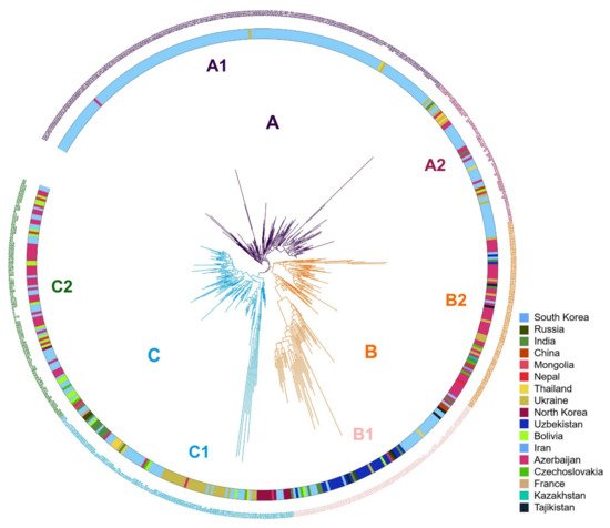
Figure 2. Phylogenetic tree for the three subgroups. Three clusters (A–C, indicated on branches) were identified, comprising a total of six subclusters with distinct geographical distributions and agronomic traits.
| C2 | ||||||||
| 8.71 ± 2.18 | ||||||||
| 26.81 ± 3.79 | ||||||||
| 99.32 ± 5.36 | 22.42 ± 5.51 | 4.76 ± 1.59 | 1.71 ± 0.63 | 80.4 ± 21.59 | ||||
| 0.9844 | ||||||||
| SSR-458 | ||||||||
| 5 | ||||||||
| 4 | ||||||||
| 0.1054 | ||||||||
| 0.0035 | ||||||||
| 0.0375 | ||||||||
| 0.0452 | ||||||||
| 0.0371 | ||||||||
| 0.981 | ||||||||
| SSR-460 | ||||||||
| 5 | ||||||||
| 3 | ||||||||
| 0.1505 | ||||||||
| 0.0035 | 0.0575 | 0.0742 | 0.0533 | 0.9723 | ||||
| Mean | 4.7838 | 4.0811 | 0.387 | 0.0032 | 0.19 | 0.4545 | 0.1735 | 0.874 |
| St. Dev | 2.7226 | 1.3829 | 0.3434 | 0.0108 | 0.1954 | 0.1928 |
a Number of genotypes in which each locus amplified alleles; b observed number of alleles; c Shannon’s information index; d observed heterozygosity; e Nei’s (1973) gene diversity; f polymorphism information content; g major allele frequency.
a Number of branches per plant; b heading date (days after sowing); c harvest time (days after sowing); d panicle length (cm); e panicle width (cm); f stem diameter (cm); g plant height (cm).
4.2. Association Analysis
The results showed high-level LD. This may be due to the mating system (selfing) of proso millet affecting the pattern of LD [29]. We arranged the TPC and SOD data corresponding to each accession on the outer circle with a simple bar (Figure S3). We observed that two red clades had higher TPCs, with average values of 25.4 and 23.2 μg/g. Blue clades had lower TPCs, with average values of 25.4 and 23.2 μg, respectively. Each clade can be clustered together because some SSR markers have the same amplification length. Therefore, we speculate that certain markers may be linked to the quantitative trait loci (QTL) associated with TPC. Comparison of the genotypes in these 4 clades showed high TPC in the 261-bp SSR-195 marker, and low TPC in the 269-bp SSR-195 marker (Supplementary Dataset 4). To further explore the relationships between these phenotypes and markers, we performed an association analysis of the phenotype and genotype data. Because proso millet is a selfed species, in the results of genetic differentiation analysis, a high degree of differentiation was observed in the population. This may lead to false positives in the association results. We choose to use the mixed linear model (MLM) for correlation analysis. In the MLM (Q + K) model, the population structure matrix (Q) and the kinship matrix (K) are used as random effects to control the false positives. SSR-31 associated with TPC explained >7.1% of the variance in TPC, indicating that there may be QTLs on both sides of the marker.
There have been a large number of reports on the antioxidant mechanism of total phenols. The number and position of hydroxyl groups in phenolic compounds, and the nature of the substituents on the aromatic ring, determine the antioxidant capacity of plant extracts [30]. Whole-genome sequencing of the proso millet genome has been completed [31]. In future research, we will map the positions of SSR-31 identified in this study on the proso millet genome and develop flanking markers to gradually narrow the target range and determine the main proso millet genes influencing TPC and oxidation capacity, and clarify the types of phenolic compounds and antioxidant mechanisms in this species. This will provide new opportunities for high-quality proso millet breeding.