Due to the high degree of intermittency of renewable energy sources and the growing interdependences amongst formerly separated energy pathways, the modeling of adequate energy systems is crucial to evaluate existing energy systems and to forecast viable future ones. However, this corresponds to the rising complexity of energy system models (ESMs) and often results in computationally intractable programs. To overcome this problem, time series aggregation is frequently used to reduce ESM complexity. As these methods aim at the reduction of input data and preserving the main information about the time series, but are not based on mathematically equivalent transformations, the performance of each method depends on the justifiability of its assumptions.
- time series aggregation
- complexity reduction
- energy system model
- temporal resolution
- renewable energy systems
- clustering
- typical days
- time slices
- system states
- snapshots
Note: The entry will be online only after author check and submit it.
1. Introduction
2. Time Series Aggregation
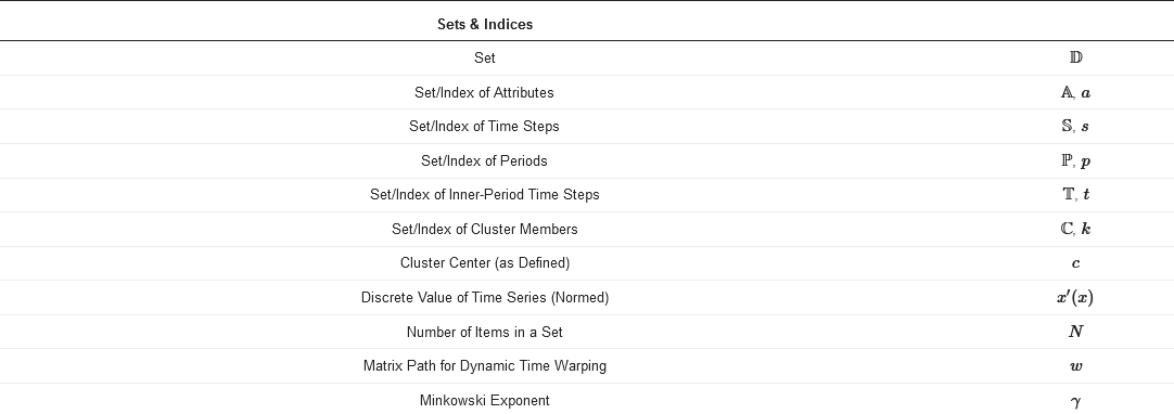
The following section deals with the general concept of TSA. For the mathematical examinations of the following section, the nomenclature of Table 1 is used.
Table 1. Nomenclature for the mathematical examinations in the following section.
The input data D usually consists of one time series for each attribute, i.e., D=A×S. The set of attributes A describes all types of parameters that are ex-ante known for the energy system, such as the capacity factors of certain technologies at certain locations or demands for heat and electricity that must be satisfied. The set of time steps describes the shape of the time series itself, i.e., sets of discrete values that represent finite time intervals, e.g., 8760 time steps of hourly data to describe a year. For all methods presented in the following, it is crucial that the time series of all attributes have identical lengths and TR. The possible shape of this highly resolved input data is shown in the left upmost field in Figure 2.
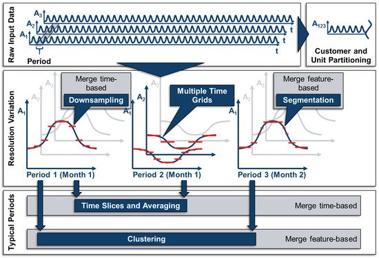
Figure 2. Methods of time series aggregation (TSA) for energy system models (ESMs).
One approach for aggregating the input time series is to merge multiple time series of attributes with a similar pattern. However, this can only be performed for attributes describing similar units (e.g., the capacity factors of similar wind turbines) or similar customer profiles (i.e., the electricity demand profiles of residential buildings). As this approach is often chosen to merge spatially distributed but similar technologies, it is not considered as TSA in the narrow sense, but as spatial or technological aggregation, as the number of time steps is not reduced in these cases. This is illustrated in the right upmost field in Figure 2.
TSA, as it is understood in this review, is the aggregation of redundant information within each time series, i.e., in the case of discrete time steps, the reduction of the overall number of time steps. This can be done in several ways. One way of reducing the number of time steps, as is shown in the central field of Figure 2, is the merging of adjacent time steps. Here, it needs to be highlighted that the periods shown in this field are for illustrative purposes only: The merging of adjacent time steps can be performed for full-length time series or time periods of time series only. Moreover, the merging of adjacent time steps can either be done in a regular manner, e.g., every two time steps are represented by one larger time step (downsampling) or in an irregular manner according to, e.g., the gradients of the time series (segmentation). A third possible approach is to individually variate the temporal resolution for each attribute, i.e., using multiple time grids, which could also be done in an irregular manner, as pointed out by Renaldi et al. [61].
Another approach for TSA is based on the fact that many time series exhibit a fairly periodic pattern, i.e., time series for solar irradiance have a strong daily pattern. In the case of perfect periodicity, a time series could thus be represented by one period and its cardinality without the loss of any information. Based on this idea, time series are often divided into periods as already shown in the middle of Figure 2. As the periods are usually not constant throughout a year (e.g., the solar irradiance is higher in the summer than in the winter), the periods can either be merged based on their position in the calendar (time slices and averaging) or based on their similarity (clustering), as shown at the bottom of Figure 2.
In the following, methods that merge time steps or periods in a regular manner, i.e., based on their position in the time series only, will be referred to as time-based methods, whereas aggregation based on the time steps’ and periods’ values will be called feature-based. In this context, features refer not only to statistical features as defined by Nanopoulos et al. [62], but in a broader sense to information inherent to the time series, regardless of whether the values or the extreme values of the time series themselves or their statistical moments are used [63].
2.1. Resolution Variation
The simplest and most intuitive method for reducing the data volume of time series for ESMs is the variation of the TR. Here, three different procedures can be distinguished that have been commonly used in the literature:
2.1.1. Downsampling
Downsampling is a straightforward method for reducing the TR by representing a number of consecutive discrete time steps by only one (longer) time step, e.g., a time series for one year of hourly data is sampled down to a time series consisting of 6 h time steps. Thus, the number of time steps that must be considered in the optimization is reduced to one sixth, as demonstrated by Pfenninger et al. [37]. As the averaging of consecutive time steps leads to an underestimation of the intra-time step variability, capacities for RES tend to be underestimated because their intermittency is especially weakly represented [37]. Figure 3 shows the impact of downsampling the PV profile from hourly resolution to 6-h time steps, resulting in one sixth of the number of time steps. In comparison to the original time series, the underestimation of extreme periods is remarkable. This phenomenon also holds true for sub-hourly time steps [38,64,65] and, for instance, in the case of an ESM containing a PV cell and a battery for a residential building, this not only has an impact on the built capacities, but also on the self-consumption rate [38,65]. For wind, the impact is comparable [64]. As highlighted by Figure 2, downsampling can also be applied to typical periods. To the best of our knowledge, this was initially evaluated by Yokoyama et al. [66] with the result that it could be a crucial step to resolve a highly complex problem, at least close to optimality. The general tendency of downsampling to underestimate the objective function was shown in a subsequent work by Yokoyama et al. [67] and the fact that this is not necessarily the case when combined with other methods in a third publication [68].
Figure 3. The time series of photovoltaic capacity factors downsampled to 1460 6 h time steps.
2.1.2. Segmentation
In contrast to downsampling, segmentation is a feature-based method of decreasing the TR of time series with arbitrary time step lengths. To the best of our knowledge, Mavrotas et al. [54] were the first to present an algorithm for segmenting time series to coarser time steps based on ordering the gradients between time steps and merging the smallest ones. Fazlollahi et al. [69] then introduced a segmentation algorithm based on k-means clustering in which extreme time steps were added in a second step. In both works, the segmentation methods were applied to typical periods, which will be explained in the following chapters. Bungener et al. [70] used evolutionary algorithms to iteratively merge the heat profiles of different units in an industrial cluster and evaluated the different solutions obtained by the algorithm with the preserved variance of the time series and the sum of zero-flow rate time steps, which indicated that a unit was not active. Deml et al. [71] used a similar, but not feature-based approach, as Mavrotas et al. and Fazlollahi et al. [54,69] for the optimization of a dispatch model. In this approach, the TR of the economic dispatch model was more reduced the further time steps lay in the future, following a discretized exponential function. Moreover, they compared the results of this approach to those of a perfect foresight approach for the fully resolved time horizon and a model-predictive control and proved the superiority of the approach, as it preserved the chronology of time steps. This was also pointed out in comparison to a typical periods approach by Pineda et al. [72], who used the centroid-based hierarchical Ward’s algorithm [73] with the side condition to only merge adjacent time steps. Bahl et al. [74], meanwhile, introduced a similar algorithm as Fazlollahi et al. [69] inspired by Lloyd’s algorithm and the partitioning around medoids algorithm [75,76] with multiple initializations. This approach was also utilized in succeeding publications [77,78]. In contrast to the approach of Bahl et al. [74], Stein et al. [79] did not use a hierarchical approach, but formulated an MILP in which not only extreme periods could be excluded beforehand, but also so that the grouping of too many adjacent time steps with a relatively small but monotone gradient could be avoided. The objective function relies on the minimization of the gradient error, similar to the method of Mavrotas et al. [54]. Recently, Savvidis et al. [80] investigated the effect of increasing the TR at times of the zero-crossing effect, i.e., at times when the energy system switches from the filling of storages to withdrawing and vice versa. This was compared to the opposite approach, which increased resolution at times without zero crossing. They also arrived at the conclusion that the use of irregular time steps is effective for decreasing the computational load without losing substantial information. Figure 4 shows advantages of the hierarchical method proposed by Pineda et al. [72] compared to the simple downsampling in Figure 3. The inter-daily variations of the PV profile are much more accurately preserved choosing 1460 irregular time steps compared to simple downsampling with the same number of time steps.
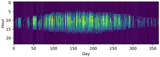
Figure 4. The time series of photovoltaic capacity factors segmented to 1460 time intervals using hierarchical merging of adjacent time steps based on centroids as proposed by Pineda et al. [72].
2.1.3. Multiple Time Grids
The idea of using multiple time grids takes into account that different components that link different time steps to each other, such as storage systems, have different time scales on which they operate [14,15,81]. For instance, batteries often exhibit daily storage behavior, whereas hydrogen technologies [14,15] or some thermal storage units [81,82] have seasonal behavior. Because of this, seasonal storage is expected to be accurately modeled with a smaller number of coarser time steps. Renaldi et al. [61] applied this principle to a solar district heating model consisting of a solar thermal collector, a backup heat boiler, and a long- and a short-term thermal storage system to achieve the optimal tradeoff between the computational load and accuracy for modeling the long-term thermal storage with 6 h time steps and the remaining components with hourly time steps. It is important to highlight that the linking of the different time grids was achieved by applying the operational state of the long-term storage to each time step of the other components if they lay within the larger time steps of the long-term storage. This especially reduced the number of binary variables of the long-term storage (because it could not charge and discharge at the same time). However, increasing the step size led to an even further increase in calculation time, as the operational flexibility of the long-term storage became too stiff and the benefit from reducing the number of variables of the long-term storage decreased. Thus, this method requires knowledge about the characteristics of each technology beforehand. Reducing the TR of single components is a highly demanding task and is left to future research.
2.2. Typical Periods
The aggregation of time series into typical periods is based on the idea that energy systems behave similarly under similar external conditions, e.g., similar energy demands and capacity factors of RES [83]. Typical periods can consist of single time steps, which are called “system states” [19,83,84,85,86], “snapshots” [63,87], or “external operation conditions” [88] in the literature, or periods containing more than one time step, e.g., “typical days” (TDs) or “representative days”, which were used by the majority of authors. In the context of control engineering, the term “system states” is especially misleading, as the state of a system not only depends on external parameters such as capacity factors and demands to be fulfilled, but also on storage levels and other endogenous state variables. Therefore, the term “system state” in discrete ESMs is only equivalent to time steps if the system is not temporally coupled, i.e., neither state variables, nor intertemporal constraints linking them with each other exist. The following will refer to “typical time steps” (TTSs) if the typical period consists of only one time step. If not stated differently in the following, the authors used TDs. However, longer periods such as typical (also called representative) weeks ([57,89,90,91] (“typical weeks”), [92,93,94,95] (“representative weeks”) also exist. This work only makes further use of the word “representative” in the context of clustering, as the representative of each cluster [96] is then interpreted as the new typical period.
Analogous to the previous chapter, a number of time-based and feature-based methods exist that will be explained in the following.
2.2.1. Time-Based Merging
Time-based approaches of selecting typical periods rely on the modeler’s knowledge of the model. This means that characteristics are included that are expected to have an impact on the overall design and operation of the ESM. As will be shown in the following, this was most frequently done for TDs, although similar approaches for typical weeks [89] or typical hours (i.e., TTSs) [97] exist. As pointed out by Schütz et al. [58], the time-based selection of typical periods can be divided into month-based and season-based methods, i.e., selecting a number of typical periods from either each month or from each season. However, we divide the time-based methods in consecutive typical periods and non-consecutive typical periods that are repeated as a subset with a fixed order in a pre-defined time interval.
2.2.1.1. Averaging
The method that is referred to as averaging in the following, as per Kotzur et al. [57], focuses on aggregating consecutive periods into one period. To the best of our knowledge, this idea was first introduced by Marton et al. [98], who also introduced a clustering algorithm that indicated whether a period of consecutive typical periods of Ontario’s electricity demand had ended or not. In this way, the method was capable of preserving information about the order of TDs. However, it was not applied to a specific ESM. In contrast to that method, one TD for each month at hourly resolution, resulting in 288 time steps, was used by Mavrotas et al. [54], Lozano et al. [99], Schütz et al. [100], and Harb et al. [101]. Although thermal storage systems have been considered in the literature [99,100,101] (as well as a battery storage by Schütz et al. [100]), they were constrained to the same state of charge at the beginning and end of each day. The same holds true in the work of Kotzur et al. [57]. Here, thermal storage, batteries and hydrogen storage were considered and the evaluation was repeated for different numbers of averaged days. Buoro et al. [89] used one typical week per month to simulate operation cycles on a longer time scale. Kools et al. [102], in turn, clustered eight consecutive weeks in each season to one TD with 10 min resolution, which was then further down-sampled to 1 h time steps. The same was done by Harb et al. [101], who compared twelve TDs of hourly resolution to time series with 10 min. time steps and time series down-sampled to 1 h time steps. This illustrates that both methods, downsampling and averaging, can be combined. Voll et al. [103] aggregated the energy profiles even further with only one time step per month, which can also be interpreted as one TD per month down-sampled to one time step. To account for the significant underestimation of peak loads, the winter and summer peak loads were included as additional time steps. Figure 5 illustrates the impact of representing the original series by twelve monthly averaged consecutive typical days, i.e., 288 time steps instead of 8760.
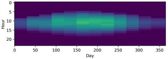
Figure 5. The time series of photovoltaic capacity factors represented by twelve monthly averaged periods as used in other studies [54,99,100] and reproduced by Kotzur et al. [57] using the python package tsam [57] (i.e., 288 different time steps).
2.2.1.2. Time Slices
To the best of our knowledge, the idea of time slices (TSs) was first introduced by the MESSAGE model [9,51] and the expression was reused for other models, such as THEA [104], LEAP [105], OSeMOSYS [106], Syn-E-Sys [107], and TIMES [48,49]. The basic idea is comparable to that of averaging, but not based on aggregating consecutive periods. Instead, TSs can be interpreted as the general case of time-based grouping of periods. Given the fact that electricity demand in particular not only depends on the season, but also on the weekday, numerous publications have used the TS method for differentiating between seasons and amongst days. In the following, this approach is referred to as time slicing, although not all of the cited publications explicitly refer to the method thus. Instead, the method is sometimes simply called “representative day” [66,67,108,109,110,111,112,113], “TD” [54,114,115,116,117,118,119,120,121], “typical daily profiles” [16,17], “typical segment” [122] “time slot” [52], or “time band” [123]. Accordingly, the term “TS” is used by the majority of authors [36,39,51,104,105,106,107,124,125,126,127,128]. The most frequent distinction is made between the four seasons [16,17,36,39,104,105,106,107,115,121,124,126,127,128] or between summer, winter. and mid-season [40,51,54,66,67,91,108,109,110,112,117,118,120,123,129,130], but other distinctions such as monthly, bi-monthly, or bi-weekly among others [40,51,54,111,113,114,116,119,122,125] can also be found. Within this macro distinction, a subordinate distinction between weekdays and weekend days [16,17,51,106,107,111,113,116,121,122,123], weekdays, Saturdays, and Sundays [115,124,126], Wednesdays, Saturdays, and Sundays [104,105], or others, such as seasonal, median, and peak [40] can be found. In contrast to the normal averaging, each TS does not follow the previous one, but is repeated in a certain order a certain number of times (e.g., five spring workdays are followed 13 times by two weekend spring days before the summer periods follow). As a visual inspection of Figure 5 and Figure 6 shows, the TS method relying on the distinction between weekdays and seasons is not always superior to a monthly distinction. The reason for this is that some input data such as the PV profile from the example have no weekly pattern and spacing the typical periods equidistantly is the better choice in this case if no other input time series (such as, e.g., electricity profiles) must be taken into account. Thus, the choice of the aggregation method should refer to the pattern of the time series considered to be especially important for the ESM. For instance, the differences between week- and weekend days is likely more important to an electricity system based on fossil fuels and without storage technologies, whereas an energy system based on a high share of RES, combined heat and power technologies, and storage units is more affected by seasonality.
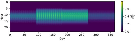
Figure 6. The time series of photovoltaic capacity factors represented by twelve time slices (TSs) (average Wednesday, Saturday and Sunday for each season) as used by Nicolosi et al. and Haydt et al. [104,105] (i.e., 288 different time steps).
2.2.1.3. Time Slices/Averaging + Downsampling/Segmentation
Like the simple averaging of consecutive time periods that can be further sampled down, e.g., as done by Harb et al. [101], the typical periods in the TS method can also be further sampled down. This can be done, for instance, by downsampling to 2 h TSs [116,118,122], 4 h TSs [40], or a number of different time step sizes to investigate the downsampling impact [66,67,68]. Moreover, day and night cycles (two diurnal TSs) [36,104,126,127,128], optionally including the peak hour of the day [36,127,128] or other TSs of irregular length [39,54,106,107,112,123,129], were also used. Mavrotas et al. [54] also implemented an algorithm for segmenting the chosen TDs to coarser TSs based on ordering of the gradients between time steps and merging the smallest ones.
The extreme case of both the downsampling method and averaging/TS method is the representation of the total time series by its mean, which was performed by Merrick et al. [40]. As this approach is unable to consider any dynamic effects, it only served as a benchmark.
2.2.2. Feature-Based Merging
In contrast to representing time series with typical periods based on a time-based method, typical periods can also be chosen on the basis of features. In this section, the clustering procedure is explained both conceptually and mathematically. To the best of our knowledge, one of the first and most frequently cited works by Domínguez-Muñoz et al. [55] used this approach to determine typical demand days for a CHP optimization, i.e., an energy system optimization model with discrete time steps, even though it was not applied to a concrete model in this work. For this purpose, all time series are first normalized to encounter the problem of diverse attribute scales. Then, all time series are split into periods P, which are compared to each other by transforming them for each value x of each attribute a at each time step t
within the period to a hyper-dimensional data point. Those data points with low distances to each other are grouped into clusters and represented by a (synthesized or existing) point within that cluster considered to be a “typical” or “representative” period. Additionally, a number of clustering algorithms are not centroid-based, i.e., they do not preserve the average value of the time series [58] which could, e.g., lead to a wrong assumption of the overall energy amount provided by an energy system across a year. To overcome this problem, time series are commonly rescaled in an additional step. The methods for this are presented in Sub-Section 3.2.2.3. This means that time series clustering includes five fundamental aspects:
- A normalization (and sometimes a dimensionality reduction).
- A distance metric.
- A clustering algorithm.
- A method to choose representatives [59].
- A rescaling step in the case of non-centroid based clustering algorithms.
As the clustered data are usually relatively sparse, while the number of dimensions increases with the number of attributes, the curse of dimensionality may lead to unintuitive results incorporating distance metrics [131], such as the Euclidean distance [59,132,133,134]. Therefore, a dimensionality reduction might be used in advance [135,136,137], but is not further investigated in this work for the sake of brevity. In the following, each of the bullet points named above will be explained with respect to their application in TSA for ESMs. Further, the distance metric, clustering method, and the choice of representatives will jointly be presented in Section 3.2.2.2, because the number of clustering methods used for ESMs is small. Figure 6 shows the mandatory steps for time series clustering used for ESMs, which are presented in the following. Figure 7 shows the time series of photovoltaic capacity factors represented by 12 typical days (TDs) using k-means clustering and the python package tsam [57].
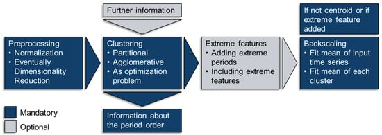
Figure 6. Steps for clustering time series for energy system models (ESMs).
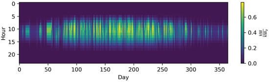
Figure 7. The time series of photovoltaic capacity factors represented by twelve typical days (TDs) using k-means clustering and the python package tsam [57] (i.e., 288 different time steps).
2.2.2.1. Preprocessing and Normalization
Clustering normally starts with preprocessing the time series, which includes a normalization step, an optional dimensionality reduction and an alignment step. Because of the diversity of scales and units amongst different attributes, they must be normalized before applying clustering algorithms to them. Otherwise, distance measures used in the clustering algorithm would focus on large-scaled attributes and other attributes would not be properly represented by the cluster centers. For example, capacity factors are defined as having values of between zero and one, whereas electricity demands can easily reach multiple gigawatts. Although a vast number of clustering algorithms exist, the min-max normalization is used in the majority of publications [14,18,39,57,58,69,92,93,135,138,139,140,141]. For the time series of an attribute a∈A={1,…,Na}consisting of s∈S={1,…,Ns} time steps, the normalization to the values assigned to a in time step s is calculated as follows:
xa,s=x′a,s−min(x′a)max(x′a)−min(x′a)(1)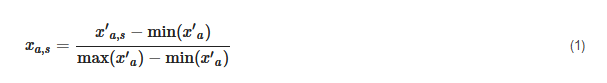
In cases in which the natural lower limit is zero, such as time series for electricity demands, this is sometimes [37,86,88,94,142,143,144,145] reduced to:
xa,s=x′a,smax(x′a)(2)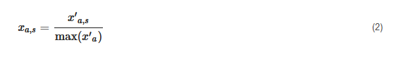
Another normalization that can be found in the literature [41,97,146,147,148] is the z-normalization that directly accounts for the standard deviation, rather than for the maximum and minimum outliers, which implies a normal distribution with different spreads amongst different attributes:
xa,s=x′a,s−x¯′aσ(x′a)(3)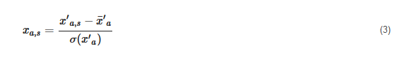
In the following, the issue of dimensionality reduction will not be considered due to the fact that it is only used in a small number of publications [135,136,137] and transforms the data into eigenvectors to tackle the non-trivial behavior of distance measures used for clustering in hyper-dimensional spaces [133].
A time series can further be divided into a set of periods P and a set of time steps within each period T, i.e., S=P×T. The periods are clustered into non-overlapping subsets PC, which are then represented by a representative period, respectively. A representative period consists of at least one discrete time step and, depending on the number and duration of time steps, it is often referred to as a typical hour, snapshot or system state, typical or representative day, or typical week. The data D=A×P×T can thus be rearranged so that each period is represented by a row vector in which all inter-period time steps of all attributes are concatenated, i.e.,
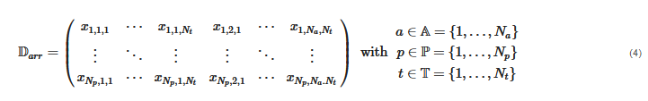
The row vectors of Darr are now grouped with respect to their similarity. Finally, yet importantly, it must be highlighted that the inner-period time step values can also be sorted in descending order, which means that, in this case, the duration curves of the periods are clustered as done in other studies [18,140,149,150]. This can reduce the averaging effect of clustering time series without periodic patterns such as wind time series.
2.2.2.2. Algorithms, Distance Metrics, Representation
Although a vast number of different clustering algorithms exist [96,151] and have been used for time series clustering in general [59], only a relatively small number of regular clustering algorithms have been used for clustering input data for energy system optimization problems, which will be presented in the following. Apart from that, a number of modified clustering methods have been implemented in order to account for certain properties of the time series, which will be part of Section 3.2.3. The goal of all clustering methods is to meaningfully group data based on their similarity, which means minimizing the intra-cluster difference (homogeneity) or maximizing the inter-cluster difference (separability) or a combination of the two [152]. However, this depends on the question of how the differences are defined. To begin with, the clustering algorithms can be separated into partitional and deterministic hierarchical algorithms.
Partitional Clustering
One of the most common partitional clustering algorithms used in energy system optimization is the k-means algorithm, which has been used in a variety of studies [14,15,24,37,57,58,63,69,74,78,83,84,85,86,87,97,137,138,139,141,142,145,146,147,148,153,154,155,156,157,158,159,160,161]. The objective of the k-means algorithm is to minimize the sum of the squared distances between all cluster members of all clusters and the corresponding cluster centers, i.e.,
min∑k=1Nk∑p∈Ckdist(xp,ck)2(5)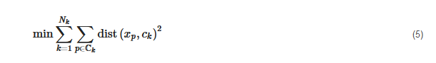
The distance metric in this case is the Euclidean distance between the hyperdimensional period vectors with the dimension dim(vec(T×A))
and their cluster centers ck, i.e.,
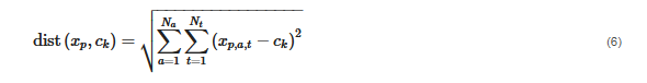
where the cluster centers are defined as the centroid of each cluster, i.e.:
ck=1|Ck|∑p∈Ckxp,a,t(7)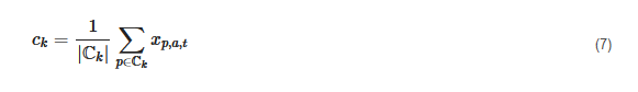
This NP-hard problem is generally solved by an adopted version [76] of Lloyd’s algorithm [75], a greedy algorithm that heuristically converges to a local minimum. As multiple runs are performed in order to improve the local optimum, improved versions (such as k-means++) for setting initial cluster centers have also been proposed in the literature [162].
The only difference regarding the k-medoids algorithm is that the cluster centers are defined as samples from the dataset that minimize the sum of the intra-cluster distances, i.e., that are closest to the clusters’ centroids.
ck=argminxl∈Ck1Nk∑p∈Ckdist(xp,xl)2(8)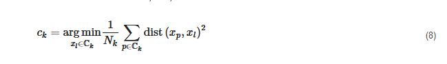
This clustering algorithm was used by numerous authors [14,19,41,55,57,58,74,78,86,139,141,149,150,159,163,164,165,166,167], either by using the partitioning around medoids (PAM) introduced by Kaufman et al. [168] or by using an MILP formulation introduced by Vinod et al. [169] and used in several studies [14,41,55,57,139,159,164]. The MILP can be formulated as follows:
min∑i=1Np∑j=1Npdist(xi,xj)×zi,j(9)
Subject to:
∑j=1Npzi,j=1 ∀ j∈1,…,Ni(10)
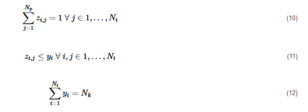
zi,j≤yi ∀ i,j∈1,…,Ni(11)
∑i=1Niyi=Nk(12)
In a number of publications [41,57,58,86,139,141,159], k-medoids clustering was directly compared to k-means clustering. The general observation is that k-medoids clustering is more capable of preserving the intra-period variance, while k-means clustering underestimates extreme events more gravely. Nevertheless, the medoids lead to higher root mean squared errors compared to the original time series. This leads to the phenomenon that k-medoids outperforms k-means in the cases of energy systems sensitive to high variance, as in self-sufficient buildings, e.g., as shown by Kotzur et al. [57] and Schütz et al. [139]. In contrast to that, k-means outperforms k-medoids clustering in the case of smooth demand time series and non-rescaled medoids that do not match the overall annual demand in the case of k-medoids clustering, as shown by Zatti et al. [141] for the energy system of a university campus.
Agglomerative Clustering
In contrast to partitional clustering algorithms that iteratively determine a set consisting of k clusters in each iteration step, agglomerative clustering algorithms such as Ward’s hierarchical algorithm [73] stepwise merge clusters aimed at minimizing the increase in intra-cluster variance
SSE=∑p∈Ckdist(xp,ck)2(13)
in each merging step until the data is agglomerated to k clusters. The algorithm is thus deterministic and does not require multiple random starting point initializations. Analogously to k-means and k-medoids, the cluster centers can either be represented by their centroids [41,159] or by their medoids [18,37,41,57,72,86,135,140,143,144,148,159]. The general property that centroids underestimate the intra-period variance more severely due to the averaging effect is equivalent to the findings when using k-means instead of k-medoids.
Rarely Used Clustering Algorithms
Apart from the frequently used clustering algorithms in the literature, two more clustering algorithms were used in the context of determining typical periods based on unsorted time intervals of consistent lengths.
K-medians clustering is another partitional clustering algorithm that is closely related to the k-means algorithm and has been used in other studies [58,139]. Taking into account that the Euclidean distance is only the special case for of the Minkowski distance [170]
dist(xp,ck)=(∑a=1Na∑t=1Nt|xp,a,t−ck|γ)1γ(14)
K-medians generally tries to minimize the sum of the distances of all data points to their cluster center in the Manhattan norm, i.e., for γ=1
and the objective function [171,172]:
min∑k=1Nk∑p∈Ckdist(xp,ck) with dist(xp,ck)=∑a=1Na∑t=1Nt|xp,a,t−ck|(15)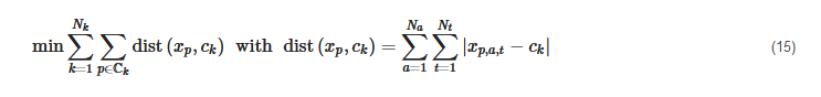
For this, the L1 distance is usually used in the assignment step [171] and the median is calculated in each direction to minimize the L1 distance within each cluster [172]. However, Schütz et al. [58,139] used the Euclidean distance (like for k-means) in the assignment step to isolate the influence of using dimension-wise medians instead of dimension-wise means (i.e., centroids). Thus, all values come from the original dataset, but not necessarily from the same candidates [58].
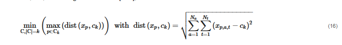
Moreover, Schütz et al. [58,139] used k-centers clustering, which minimizes the maximum distance of all candidates to its cluster center, i.e., according to Har-Peled [173],
Time Shift-Tolerant Clustering Algorithms
The last group of clustering algorithms applied for TSA in ESMs is time shift-tolerant clustering algorithms. These algorithms not only compare to the values of different time series at single time steps (pointwise), but also compare values along the time axis with those of other time series (pairwise). In the literature [41,159], dynamic time warping (DTW) and the k-shape algorithm are used, both of which are based on distance measures that are not sensitive to phase shifts within a typical period, which is the case for the Euclidean distance. The dynamic time-warping distance is defined as:
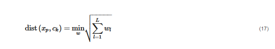
where w describes the so-called warping path, which is the path of minimal deviations across the matrix of cross-deviations between any entry of xp and any entry of ck [41,174]. The cluster centers ck are determined using DTW Barycenter averaging, which is the centroid of each time series value (within an allowed warping window) assigned to the time step [175]. Moreover, a warping window [41,159] can be determined that limits the assignment of entries across the time steps. Shape-based clustering uses a similar algorithm and tries to maximize the cross-correlation amongst the periods. Here, the distance measure to be minimized is the cross-correlation and the period vectors are uniformly shifted against each other to maximize it [41,159,174,176]. It must be highlighted that both dynamic time warping and shape-based distance, have only been applied on the clustering of electricity prices, i.e., only one attribute [41,159]. Moreover, Liu et al. [148] also applied dynamic time warping to demand, solar, and wind capacity factors simultaneously. However, it is unclear how it was guaranteed that different attributes were not compared to each other within the warping window which remains a field of future research. Furthermore, a band distance, which is also a pairwise rather than a pointwise distance measure, was used in a k-medoids algorithm by Tupper et al. [167], leading to significantly less loss of load when deriving operational decisions for the next day using a stochastic optimization model.
2.2.2.3. Rescaling
Due to the fact that not all of the methods rely on the representation of each cluster by its centroid (i.e., the mean in each dimension), these typical periods do not meet the overall average value when weighted by their number of appearances and must be rescaled. This also holds true for the consideration of extreme periods, which will be explained in the following chapters. Accordingly, the following section will be referred to if rescaling is considered in the implementation of extreme periods. To the best of our knowledge, the first work that used clustering not based on centroids was that of Domínguez-Muñoz et al. [55], in which the exact k-medoids approach was chosen as per Vinod et al. [169]. Here, each attribute (time series) of each TD was rescaled to the respective cluster’s mean, i.e.,
c∗k,a,t=ck,a,t∑p∈Ck∑Ntt=1xp,a,t|Ck|∑Ntt=1ck,a,t ∀ k,a,t(18)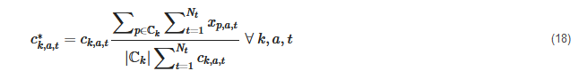
Furthermore, Domínguez-Muñoz et al. [55] discarded the extreme values that were manually added from the rescaling procedure. A similar procedure, which was applied for each time series, but not for each TD, was introduced by Nahmmacher et al. [143], who used hierarchical clustering based on Ward’s algorithm [73] and chose medoids as representatives, which was later used in a number of other studies [14,18,41,57,140,159]. Here, all representative days were rescaled to fit the overall yearly average when multiplied by their cardinality and summed up, but not the average of their respective clusters, i.e.,
c∗k,a,t=ck,a,t∑Npp=1∑Ntt=1xp,a,t∑Nkk=1(|Ck|∑Ntt=1ck,a,t) ∀ k,a,t(19)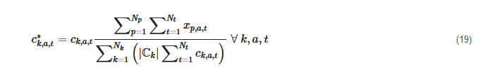
Schütz et al. [58,139], Bahl et al. [74], and Marquant et al. [149,150] refer to the method of Domínguez-Muñoz et al. [55], but some used it time series-wise and not cluster- and time series-wise. Schütz et al. [58,139] were the first to highlight that both approaches are possible. It also needs to be highlighted that these methods are not the only methods, as Zatti et al. [141], for instance, presented a method to choose medoids within the optimization problem without violating a predefined maximum deviation from the original data, but for the sake of simplicity, it focused on the most frequently used post-processing approaches. Additionally, other early publications, such as by Schiefelbein et al. [163], did not use rescaling at all. Finally, yet importantly, the rescaling combined with the min-max normalization could lead to values over one. Accordingly, these values were reset to one so as to not overestimate the maximum values and the rescaling process was re-run in several studies [14,18,57,140,143]. In contrast, Teichgräber et al. [41,159] used the z-normalization with rescaling in accordance with Nahmmacher et al. [143], but did not assure that the original extreme values were not overestimated by rescaling.
2.2.3. Modified Feature-Based Merging
Apart from the methods that are based on the direct clustering of the time series’ values or periods, a number of methods exist that group time series in a consecutive manner [53], by means of other features, such as sorted time series (i.e., duration curves) [18,20,92,93,94,95,140,144,149,150,177] or other statistical features such as the average, variance, minimal and maximal values [63], or predefine the clusters based on additional information [88]. These methods will be presented in the following.
With respect to grouping consecutive typical periods, an early publication by Balachandra et al. [53] started by grouping daily residual load profiles by month, and then applied multiple discriminant analysis to these groups and reclassified the days at the beginning or end of a group (month) to the preceding or subsequent group if they were more similar to it. This resulted in nine consecutive groups represented by their centroids. However, this aggregation was not applied to an energy system optimization.
Furthermore, a number of publications [20,94,95,144] rely on the principle introduced by Poncelet et al. [177]. For this, the normalized duration curves were placed into bins, i.e., how many hours of the year surpass a certain level between zero and the maximum level of the specific attribute. The same was performed for each candidate day. Then, the sum of absolute differences between the hours at which the reference curve surpassed a bin border and the hours at which the curve derived from a linear combination of a given number of candidates surpassed the same bin borders was minimized in an MILP.
Another approach aimed at reproducing a yearly duration curve was introduced by de Sisternes et al. [92,93]. Here, the duration curve of power feed-in by wind and solar at a certain penetration level was calculated and approximated by an exhaustive search for a combination from a subset of typical weeks. As this was a combinatorial problem, the computation time rapidly increased for higher numbers of weeks. In a later publication [92], the variability of the selected weeks was used as an additional metric.
Instead of clustering the original time series, the yearly duration curve was approximated in a number of publications [18,140,149,150]. For this, the candidate days were simply sorted prior to being clustered. This decreased the averaging effect of statistical events, such as wind, as the largest value and second largest, etc. always lay in the first dimension and second dimension, etc.
With respect to the clustering of other statistical features apart from the distribution curve (duration curve), Agapoff et al. [63] applied k-means clustering to snapshots (i.e., TTSs) and used different features for the clustering: either absolute values or the average, minimum, maximum, and standard deviation of all considered regions for either price differences, non-controllable demand and generation, or both. This is an extension with promising results to all thus far used clustering algorithms only applied to normalized absolute values.
Finally, yet significantly, Lythcke-Jørgensen et al. [88] introduced a so-called CHOP-method that was based on splitting the range of each attribute, in this case the power price and relative heat demand on a five-year basis, into different intervals based on important values (e.g., zero-price) and even divisions between them. Then, all values (i.e., hours) were transferred in a 2d space in which the intervals for both attributes formed a grid. From each cell, the centroid was subsequently calculated if it contained any candidate hours. As information about the chronology of these TTSs was lost, the design of storage technologies resulted in large deviations from the reference case.
These cases highlight that methods based on well-known approaches are constantly customized for specific ESMs and improved where possible, which illustrates that the development of TSA methods is a dynamic process.
2.2.4. Linking Typical Periods
As mentioned above, some components, such as storage components of ESMs, link consecutive time steps by means of intertemporal constraints. The representation of time series by a few TDs or weeks does not generally take their order across the entire time horizon into account. This means that the modeling of filling levels is normally only possible within these typical periods with a periodic boundary condition for the state of charge. In this case, the order of typical periods no longer plays a role. On the other hand, seasonal storage cannot be sufficiently modeled by this method. Yet, this is especially important for energy systems based on a high share of RES. As per Bauer et al. [81], central solar heating plants with introduced short-term heat storages can typically supply 15–20% of the total residential heating demand. With seasonal heat storages, this fraction can be increased to about 50%. For a long period of time, the only approach to model seasonal storages was to drastically reduce TR, as by Tveit et al. [178], making it impossible to model short-term storages. To overcome this issue, different methods have been developed that take the linking of TDs into account.
As far as we know, the TIMES framework was the first to deal with linking TSs not only consecutively, but also inter-period storages that work on a larger time scale [46,47,48,49]. However, since the inter-period storages are meant to work between different years, e.g., as waste disposal sites [46], they are not linked to the intra-period storages, which only link consecutive TSs (segments) within one typical period, such as weekdays in spring.
Welsch et al. [106] and Samsatli et al. [16] independently developed a non-uniform hierarchical time discretization that is based on the selection of TSs. In two publications [16,17], Samsatli et al. chose two TDs with hourly data for both the week and weekend which was done for each season consisting of 13 weeks. This resulted in 192 time steps. For the modeling of the seasonal storage, the energy surplus across each time scale was determined and added up. As the chosen days appeared in a regular order within each season, the capacity constraints were not postulated for each time step. Instead, they were only defined for the first and last instance of each day type, the first and last week of each season, and the first and last season of each year, if a multiple year approach was chosen. Welsch et al. [106] chose a similar approach that consisted of three TSs for a workday and a weekend day in each season. However, the case study was only run with one TD with an hourly resolution.
Both approaches did not consider a self-discharge rate. The approach of Welsch et al. [106] was later developed by Timmerman et al. [107] to handle self-discharge and re-used by van der Heijde et al. [95]. Since the typical days in these publications [16,17,95,106,107] are aligned in a regular manner, the critical storage levels can only be reached at certain time steps which significantly reduces the number of side constraints. Taking the configuration used by Timmerman et al. [107] as an example, five identical workdays alternate 13 times per season with two identical weekend days. As each week consists of only two day types, of which the first is repeated five times and the second is repeated twice, the intermediate weekdays representing Tuesday, Wednesday, and Thursday cannot include critical states of charge-neither for a rising state of charge across the weekdays (the critical day would be Friday), nor for a decreasing state of charge across the weekdays (the critical day would be Monday). The same holds true for the intermediate weeks in each season. As they are repeated 13 times, either the first or last week of each season is critical with respect to the state of charge of seasonal storage and their capacity.
Similarly, but again independently, Spiecker et al. [116] developed a comparable approach that linked workdays and weekend days for every second month in an inter-day manner for pumped storage plants and an inter-month manner for large-scale storage systems in the E2M2s model. Moreover, the TDs were based on a recombining decision tree of 2 h segments and were thus capable of modeling the storage size stochastically.
Gabrielli et al. [15] developed a method to couple TDs using a function that assigns each day of the original time series to the TD it is represented by. This function is used to couple the state of charge of consecutive (typical) days in an additional equation and means that the operation of the components is modeled for a number of TDs, while the state of charge of the storages is modeled for the entire time horizon represented by a sequence of TDs. The approach was tested for a different number of TDs, as well as in a later publication [15,160].
Wogrin et al. [85] earlier proposed the same approach as Gabrielli et al. [15] for TTSs and took the information of the clustering indices, i.e., which original time step was represented by which TTS, to link TTS in order to consider start-up and shut-down costs, which was later re-used by Tejada-Arango et al. [19] for the calculation of storage levels using typical periods (days and weeks). However, in contrast to Gabrielli et al. [15], the storage levels were not constrained for each time step by Tejada-Arango et al. [19], but only at intervals of one week. Additionally, a similar method was applied to avoid unnecessary unit transitions at the border between two consecutive TDs.
Like the idea of Gabrielli et al. [15], Kotzur et al. [14] introduced a similar method of linking TDs in a chronologically correct order. Instead of directly linking each state of charge to the preceding one, the superposition principle was used to distinguish intraday and interday states of charge. Here, the interday state of charge describes the state of charge at the beginning of each day, while the intraday state of charge is defined to be zero at the beginning of each day but is defined for each hour of each TD. The sum of both values, i.e., the intraday state of charge for a given number of TDs, along with the interday state of charge, which was determined by the sum of storage level differences of each TD in the corresponding sequence, was then used to determine the storage levels at each time step. This approach was also used in later publications dealing with seasonal storage [18,140].
Another slight deviation of this method was applied by van der Heijde et al. [20], who also used the superposition principle discussed by Kotzur et al. [14] to couple TDs. However, they did not use clustering algorithms to group similar days and represented these by one TD for each cluster, but instead searched for a linear combination of days that minimized the deviation from the yearly duration curve; a procedure introduced by Poncelet et al. [144]. In contrast to clustering algorithms, this procedure did not directly lead to an assignment of original days to groups represented by single TDs. This meant that this had to be performed in a separate step. For this, a mixed integer quadratic programm (MIQP) problem was formulated that sought to minimize the sum of squared errors of each day of the original time series to the TDs. The outcome of this was a sequence of TDs that represented the original time series, which was crucial for linking the TDs in accordance with the aforementioned approach of Kotzur et al. [14]. Recently, Baumgärtner et al. [77] included the storage formulation of Kotzur et al. [14] in their rigorous synthesis of energy systems using aggregation approaches to define upper and lower bounds for the objective function with full time resolution.
The fact that a number of methods for linking typical periods were independently developed [14,15,16,85,106] shows the value of giving an overview over all of the methods employed so far.
2.3. Random Sampling
Another minor group of publications uses TSA based on random sampling. This means that the time steps or periods are randomly chosen from the original time series and considered to be representative for the entire time series. Most of the methods in the following deal with single time steps instead of periods, which is an acceptable simplification when the impact of storage capacity or other intertemporal constraints on the system design can be neglected [166].
2.3.1. Unsupervised
As with supervised random sampling methods, unsupervised random sampling methods can be applied to typical periods or single time steps. However, they appeared earlier than the supervised methods (2011 and 2012).
Ortiga et al. [179] introduced a graphical method for which a number of days from the dataset had to be defined. In a second step, the algorithm minimized the deviation between the duration curve of the original dataset and a duration curve of the chosen periods multiplied by a set of variable factors for the number of appearances of each TD.
With respect to the random sampling of time steps, Van der Weijde et al. [180] sampled 500 out of 8760 h to capture major correlations of the input data for seven regions.
However, in the years since 2012, these methods were substituted by supervised random sampling methods.
2.3.2. Supervised
Munoz et al. [181] applied supervised random sampling for 1 up to 300 daily samples out of a dataset of seven years, which were then benchmarked against the k-means clustering of typical hours. A similar method was used by Frew et al. [182], who took two extreme days and eight random days from the dataset and weighted each day so that the sum of squared errors to the original wind, solar and load distribution was minimized. This procedure was then repeated for ten different sets of different days, with the average of each optimization outcome calculated at the end. With respect to time steps, Härtel et al. [86] either systematically determined samples taking every nth element from the time series or randomly chose 10,000 random samples from the original dataset and selected the one that minimized the deviation to the original dataset with respect to moments (e.g., correlation, mean and standard variation). Another complex algorithm for representing seasonal or monthly wind time series was proposed by Neniškis et al. [51] and tested in the MESSAGE model. This approach took into account both the output distribution (duration curve) for a TD and the inter-daily variance, not to be exceeded by more than a predefined tolerance, while using a random sampling process. However, only the typical days for wind were calculated in this way, whereas the other time series (electricity and heat) were chosen using TS. Recently, Hilbers et al. [166] used the sampling method twice with different numbers of random initial samples drawn from 36 years. From a first run, the 60 most expensive random samples were taken and included in a second run with the same number of samples.
These methods are fairly comparable to the method of clustering TTSs. However, the initial selection of samples is based on random choice.
2.4. Miscellaneous Methods
Apart from the random sampling methods that cannot be systematically categorized with the scheme in Figure 1, an even smaller number of publications cannot be grouped in any way with respect to their TSA methods. For the sake of completeness, however, they are presented in the following.
Lee et al. [183] used an improved particle swarm optimization to optimize the UC of a power system with respect to fuel and outage costs. This method was based on an evolutionary algorithm that iteratively determined the “fittest” solutions and thus was quite comparable to supervised random sampling methods. However, the use of an own class of optimization algorithm is a unique feature. A similar approach to solve the UC problem of a grid-connected building with renewable energy sources and a battery was presented by Quang et al. [184]. In their work, a genetic algorithm and a particle swarm algorithm were used for different charge and discharge rates of the battery based on half-hourly time steps. It is worth mentioning that apart from these publications, a number of other works exist which use, among other methods, genetic algorithms or particle swarm algorithms to UC models. A comprehensive review on the methods to address the UC problem was given by Saravanan et al. [185]. However, these approaches are based on a survival of the fittest principle and not on a classic optimization problem so that an aggregation can only be applied by downsampling the time steps used for simulation. Moreover, these approaches are not directly applicable to combined UC and GEP models. Therefore, these methods are not further analyzed within the scope of this paper.
Xiao et al. [186] optimized the capacity of a battery and a diesel generator for an island system by searching for the optimal cut-off frequency at which the running of a diesel generator was more convenient without causing overly high fuel costs, whereas the battery capacity would be too large if it was run on a high frequency band. For this, an analysis based on discrete Fourier transform (DFT) was used, highlighting the different specific cost-dependent time scales on which different technologies operate.
More recently, Pöstges et al. [187] introduced an analytical approach to aggregate the time steps of a demand duration curve for a simple ESM without storage units and with only one energy type. Interestingly, this method led to a simplified problem formulation based on a minimum number of time steps without causing an error in the objective function. In this case, the supply technology costs are based on capacity- and operation-specific costs and the approach was inspired by an earlier work of Sherali et al. [6]. Sherali et al. proved in 1982 that the cost optimal operation of these simple systems can be interpreted as an optimization problem which is closely related to the peak load pricing theory introduced by Boiteux in 1949 [3] (English translation in 1960 [4]) and Steiner in 1957 [5].
To summarize, special methods that cannot be categorized in any way appear in an irregular manner, but can have special implications for the improvement of preexisting methods.