Wood has been used as a construction material for thousands of years, until the twentieth century, when its importance in this field was eclipsed by the appearance and development of other materials such as steel and concrete. Nevertheless, advances in new and more resistant wood-based materials characterized by environmental advantages, improved durability and resistance to aggressive environments, and earthquake resistance [1] have renewed interest in the construction of timber structures, which have definitely increased in number.

One of the most widely used wood-based products is structural laminated wood. This is formed by gluing several wood layers arranged in the direction of the grain [2]. The gluing is done with adhesives such as polyurethane and is formed in a pressing process described in the standard [3]. According to the standards [4], the wood species suitable for the manufacture of structural laminated wood are Norway spruce (Picea abies) ^[5][6][5,6], silver fir (Abies alba) [7], Scots pine (Pinus sylvestris) [8], Oregon pine (Pseudotsuga menziesii), black pine (Pinus nigra), European larch (Larix decidua), maritime pine (Pinus pinaster) [9], poplar (Populus robusta, Populus alba), radiata pine (Pinus radiata) [10], Sitka spruce (Picea sitchensis), western hemlock (Tsuga heterophylla) [11], western red cedar (Thuja plicata) and yellow cedar (Chamaecyparis nootkatensis).

As with other kinds of structures, the joints of timber structures are always one of their weakest points [12]. Indeed, the strength of the joints usually defines the load-carrying capacity of the whole structure, which is why understanding their mechanical behavior is a matter of paramount importance to structural designers and engineers in order to improve their structural possibilities and prevent them from limiting the structure’s strength ^[13][14][13,14].

Among all the possible kinds of joints used in timber structures, dowel-type joints are one of the most common connectors [15]. They basically consist of one or more cylindrical steel dowels inserted into aligned holes of different elements. The dowels transmit loads between the elements, being subjected to opposite compressive forces on the contact area with each element. This causes the dowels to work under bending moments and shear forces. There is an almost infinite number of possible configurations for dowel-type joints. For example, they can connect two, three or more timber [16], or even steel members ^[17][18][17,18]. Not only a single dowel, but also a combination of dowels can be used, in line or in a matrix distribution [19]. The dowels can work in a single or double shear. Finally, dowel action can be reinforced through different techniques: adhesives ^[20][21][20,21], split rings or shear plate connectors [22]. Another form of reinforcement is the expansive kit, which is of particular interest as a subject for study because of its intensive use and high performance with steel and concrete ^[23][24][25][23,24,25], the other two main materials used for large constructions. Especially in concrete, expansive joints have been an improvement when evolved to prefabricated kits, which have many advantages ^[26][27][26,27]: they allow quick and easy assembly in construction, reduce repair costs, obviate the need for reconditioning work or “on-site” adjustments at the joint and offer a permanent solution and, in certain cases, are reusable. In timber structures, an expansive system has been investigated in dowels constituted by overlength hollow steel tubes expanded by compression of the tube ends [28].

Therefore, it is reasonable to think that a controlled expansion of a solid dowel in a timber joint could also provide several advantages [28]: increasing the load-carrying capacity of the joint, reducing slippage of the joint, thereby increasing its stiffness, and improving the distribution of stresses in the timber parts along the hole where the dowel is located.

2. Finite Element Model

The finite element model was prepared according to the geometry, materials and loads described in the above section. The model was meshed using a combination of eight, six- and four-node volume elements (called C3D8, C3D8 and C3D4, respectively, in Abaqus). The model has 5820 elements and 8952 nodes. The model also has five parts: rod, sleeve, block, central and lateral parts. A nonlinear analysis was performed in order to take into account the evolution of the contact between the sleeve and the timber parts and the elastoplastic mechanical behavior of both materials, timber and steel. Figure 17 shows the complete model, only a quarter of which has been meshed, benefiting from the existence of two perpendicular planes of symmetry.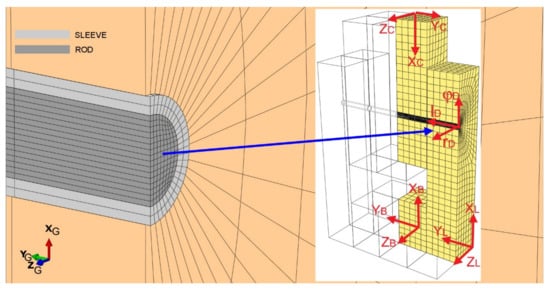 Since the development of the finite element model requires accurate specification of the directions that define the timber’s orthotropic behavior, it is necessary to consider different local coordinate systems adapted to the direction of the grain in each of the model’s timber parts. Figure 17 shows the coordinate systems used: a global one (G), three for each of the three timber parts, the central, lateral and block parts, defined as C, L and B, respectively, and a cylindrical one to study the strains and stresses in the dowel (D).

2.1. Contact Zone

The contact zone was modelled using the so-called hard formulation. In FEM contact models, the algorithm that controls the possible contact between a pair of solids requires that part of the surface of one of the solids must be defined as the master surface, and the corresponding surface of the other solid as the slave surface. The algorithm prevents the nodes of the slave surface from penetrating the master surface [15]. Moreover, it defines the force transmission between nodes when a slave surface node makes contact with the faces constructed with the master surface nodes. This force follows a step function that goes from zero, before contact, to the required value, after contact has been detected. Careful selection of mesh type and size is essential to obtain accurate contact results.

2.2. Steel and Timber Behavior Models

Steel was modelled as a homogeneous isotropic material with a 3D elastoplastic behavior described by the von Mises criterion ^[29][35], considering an effective stress-strain curve with a simplified trilinear shape ^[30][36] (symmetrical in tension and compression), with the values obtained from the results of uniaxial tests, as can be seen in Figure 28a. While the effective stress is lower than yield strength f_y it behaves as linear elastic; beyond this point, the plastic flow with isotropic hardening develops until ultimate strength f_u is reached, after which its behavior becomes perfectly plastic.

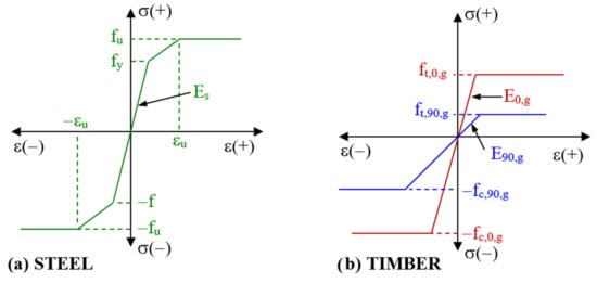
Figure 28.

Uniaxial mechanical behavior models used for: (

a

) steel and (

b

) timber.

The mechanical behavior of wood is especially difficult to simulate due to its anisotropy, which implies different elastic moduli and strengths in the different directions with respect to grain direction ^[31][32][33][37,38,39]; furthermore, the values of the latter characteristics change depending on whether it is subjected to compressive or tensile efforts. This strength asymmetry is a result of the different microscopic mechanisms that act on timber: there is fracture under tension ^[34][40] and buckling under compression in the direction of the grain, while separation of fibers under tension ^[35][41] and crushing under compression occurs in the direction perpendicular to the grain ^[36][42].

Figure 28b shows the simplified stress-strain curves considered in this work, obtained from the values indicated in Table 1, for the uniaxial behavior of the timber in the direction of the grain and perpendicular to it. The different values of the strengths in both curves and between the tension or compression branches of each one, and the different slopes of the linear elastic sections can be observed. As an approximation, and after overcoming the corresponding strengths, a perfectly plastic behavior is assumed. This results in large plastic deformations at small stress increases.

To simulate the 3D mechanical behavior of timber, it is especially important to choose a correct model that includes different values of the mechanical properties in tension or compression. Orthotropic elastoplastic models based on the Hill criterion are most widely used ^[33][39]. However, since Hill’s theory considers a symmetrical behavior in tension and compression, it is necessary to generalize it to include different characteristics of timber according to the type of effort acting on it.

2.3. User Material Subroutine for Timber

The material libraries of finite element commercial programs include the von Mises elastoplastic isotropic model, usually alongside Hill’s model for orthotropic behavior (e.g., in the program Abaqus used in this work, the latter is called Hill48), but they do not include orthotropic models that take into account the different strengths in tension and compression. However, ad hoc behavior models can be developed for most of them by using complementary procedures ^[37][38][43,44]. In Abaqus, this is done through user subroutines called UMAT, programmed in FORTRAN.

Therefore, the description of the complex mechanical behavior of timber required the development of a specific UMAT subroutine, which contains the programming of the incremental formulation of Hill’s elastoplastic model (performed following the steps indicated by certain authors ^[39][45]), but completed to use tensile or compressive strengths depending on the way in which the material is working at the analyzed point ^[40][46]. To determine how it works, the dimensionless ratios between the stresses and strengths in the three orthotropic directions are calculated, considering tensile strength if the stress is positive and compressive strength otherwise. Subsequently, the highest ratio in absolute value is determined and, if it is positive, the point is considered to work predominantly in tension; otherwise, it works in compression.

The subroutine includes the three basic stages required to define the 3D elastoplastic mechanical behavior: Hooke’s law of elastic behavior for orthotropic materials, Hill’s yield criterion to determine whether there is plastic deformation, and the associated flow rule to define the plastic behavior ^[41][47]. For each increment in deformation, Abaqus uses the subroutine at each integration point to obtain the final values of the stresses and strains after such an increment is ended. Figure 39 shows the flow chart for the subroutine. First of all, it determines whether the point is working in tension or in compression, calculating Hill´s constants with adequate strengths. Then, it assumes that the increment of deformation is elastic (elastic predictor), and the yield criterion is applied; if the criterion is not fulfilled, the increment is confirmed as elastic and the subroutine ends; otherwise the stresses and elastic and plastic strains are obtained by performing a calculation based on the flow rule (plastic corrector).

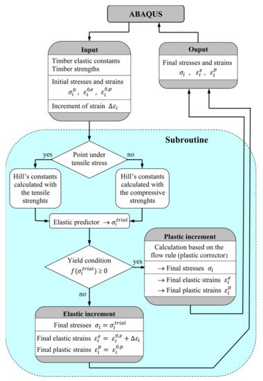
Figure 39. Flow chart of the subroutine developed for modeling the mechanical behavior of timber.

2.4. Expansion of the Dowel

After trying different ways to simulate the effect produced by the expansive kit, the procedure that seemed to have more advantages is based on exploiting the fact that finite element programs have clearly defined the mechanism of thermal expansion, which can be used to simulate the mechanical one provoked by the expansive kit. For this purpose, a thermal expansion coefficient was assigned to the rod, which was designed with an initial diameter equal to the inner diameter of the sleeve after the expansion produced by the spheres (Figure 6). A fictitious field of decreasing temperatures was established in the rod to contract it so that it could be inserted in the unexpanded steel tube that constitutes the sleeve. The second step was the elimination of the temperature field, so that the rod tries to recover its initial dimension, pushing the inner wall of the sleeve, which causes compression on the timber in the area surrounding the dowel and thus creating the expansion effect. Although this procedure seems more complicated than direct application of an expansion process, it is advantageous in that it is easier to work on the results because they do not accumulate the thermal deformations that would appear with a direct expansion process, which do not exist in the real procedure.