Your browser does not fully support modern features. Please upgrade for a smoother experience.
Please note this is a comparison between Version 1 by Bisrat Ayalew Yifru and Version 2 by Jessie Wu.
Accurate streamflow prediction (SFP) is crucial for water resource management, flood and drought forecasting, and reservoir operations. However, complex interactions between surface and subsurface processes in watersheds make predicting extreme events challenging. This work highlights the importance of incorporating physical understanding and process knowledge into data-driven SFP models for reliable and robust predictions, especially during extreme events.
- baseflow
- data-driven modeling
- streamflow prediction
- physically consistent
- hybrid modeling
1. Introduction
Streamflow—a vital element of the hydrological system—constitutes a pivotal nexus between the sustenance of diverse aquatic ecosystems and the fulfillment of fundamental human needs across agriculture, industry, and societal well-being [1][2][3][1,2,3]. It also plays a significant role in riverine processes, influencing erosion, transportation, and deposition. Additionally, streamflow serves as a critical indicator of climatic and environmental changes [4][5][4,5]. Therefore, accurate understanding and prediction of streamflow are essential for drought monitoring, infrastructure design, reservoir management, flood forecasting, water quality control, and water resource management [6][7][6,7]. However, despite advances in streamflow prediction (SFP) methods, accurate prediction remains challenging due to the complex interplay between natural and human influences on a watershed’s response to precipitation [6][8][9][10][6,8,9,10]. Land-use changes, water withdrawals, infrastructure development, topography, soil characteristics, and vegetation cover create a dynamic and interdependent system that challenges accurate modeling. Data limitations and measurement uncertainties further complicate the task [11][12][11,12].
Process-based models have been used to comprehend complex hydrological processes at the watershed scale, while data-driven modeling (DDM) has been used to predict streamflow by leveraging input–output relationships. DDM ranges from traditional statistical methods to complex artificial intelligence (AI)-based models, while process-based models encompass conceptual and physically based models [8][9][13][8,9,13]. Although less physically based, DDM often outperforms PBM in terms of predictive accuracy [14][15][16][14,15,16]. Developing physically based models is slow and requires extensive data, making DDM an attractive solution to the challenge of relating input and output variables in complex systems [17]. Moreover, DDM has the potential to avoid several sources of uncertainty in the modeling process, such as downscaling errors, hydrological model errors, and parameter uncertainty [12].
However, many operational forecasting agencies do not use DDM for SFP [18]. This may be due, in part, to the “black box” nature of DDMs, making it difficult to interpret predictions and diagnose errors [19]. Overfitting is also a significant concern in this paradigm, as the complexity of the models can lead to spurious relationships with the data [20][21][20,21]. In fact, both DDM and PBM paradigms have difficulty capturing extreme events, such as floods or prolonged droughts. While the inherent complexity and non-stationary nature of these events pose a significant challenge for any prediction model, the simplified hydrological processes often used in PBM frameworks further limit their accuracy [22]. For example, simplified representations of groundwater modules in watershed models or neglecting certain physical processes can hinder the models’ ability to capture the intricate dynamics of extreme events [23][24][23,24].
To improve SFP, several options, including domain knowledge, advanced data preprocessing techniques, multi-model integration, and metaheuristic algorithms, have been explored. While most of these techniques aim primarily to enhance prediction accuracy, PBM and domain knowledge-based approaches aim to improve prediction accuracy, interpretability, and physical consistency in a DDM framework. Incorporating domain knowledge as additional information about the mechanisms responsible for generating streamflow can help to build physically consistent models and improve model performance [14][25][26][14,25,26]. Additionally, integrating process-based models with data-driven models is recognized as a way to create a streamflow model that is both physically consistent and interpretable.
2. Overview of Basic Watershed Processes
In the modeling paradigm, particularly within the context of PBM, detailed analysis and discussion of the distinct water balance segments and hydrological processes, along with comprehensive mathematical justifications and expert insights drawn from both the water balance and intimate familiarity with a study region, are crucial for strengthening the modeling procedures. Conversely, DDM can assist in circumventing certain modeling chain steps that involve uncertainty. Given the growing prevalence of the combined data-driven and PBM approach [12][27][12,32], this section provides an overview of both methods.2.1. Streamflow Generation Processes
Several factors influence streamflow generation, such as climate, hydrogeology, soil properties, vegetation, management scenarios, and antecedent conditions. Precipitation undergoes interception by vegetation, infiltration into the soil, or surface runoff into streams. Evapotranspiration (ET) and subsurface processes, especially baseflow and lateral flow, significantly contribute to streamflow generation. From a watershed hydrology perspective, the generation is depicted based on their relation to surface processes, rootzone processes, and groundwater flow (Figure 1). However, conceptualizing and modeling streamflow has long been an intricate environmental challenge due to the significant subsurface flow mechanisms occurring in soil and bedrock, which rwesearchers have limited capacity to quantify and evaluate [28][33].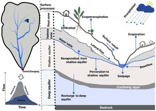
Figure 1.
Basic watershed surface and subsurface hydrological processes and simplified diagram of the hydrograph.
2.2. Streamflow Prediction
PBM is typically used when there is a good understanding of the fundamental processes driving the system, and the goal is to create a model that accurately captures those processes. On the other hand, data-driven hydrological models use statistical or soft computing methods to map inputs to outputs without considering the physical hydrological processes involved in the transformation. The DDM approach is discussed further in Section 3.3. Examples of widely utilized PBM include the Soil and Water Assessment Tool (SWAT), HBV (Hydrologiska Byråns Vattenbalansavdelning) [29][34], GR4J (Génie Rural à 4 paramètres Journalier) [30][35], Variable Infiltration Capacity (VIC) [31][36], the Hydrologic Engineering Center–Hydrologic Modeling System (HEC-HMS) [32][37], and the Precipitation-Runoff Modeling System (PRMS) [33][38]. Next, rwesearchers described the key hydrological processes and equations used in the SWAT model as an example of PBM. The SWAT model ET computation relies on potential evapotranspiration (PET) and has multiple options. The selection of a method primarily depends on the availability of data. For instance, the Penman–Monteith method [34][41] necessitates measurements of solar radiation, air temperature, relative humidity, and wind speed, whereas the Hargreaves method [35][42] requires only air temperature data.2.3. Basic Processes in Data-Driven Streamflow Prediction
DDM can be broadly classified into two types: conventional data-driven techniques and AI-based models [36][37][43,44]. Conventional techniques, such as multiple linear regression (MLR), autoregressive integrated moving average (ARIMA), autoregressive-moving average (ARMA), and autoregressive-moving average with the exogenous term (ARMAX), are preferred in SFP due to their simplicity. In contrast, AI-based models offer more advanced capabilities and higher accuracy [37][38][44,45]. The most widely utilized AI-based data-driven models fall into four categories: evolutionary algorithms, fuzzy-logic algorithms, classification methods, and artificial network techniques [10][38][10,45]. The basic steps in DDM include data preprocessing, selecting suitable inputs and architecture, parameter estimation, and model validation [39][40][41][46,47,48]. This procedure unfolds in four key steps: data collection and cleaning, feature selection and engineering, model selection and building, and prediction (Figure 2). Effective data preprocessing, which typically involves essential steps such as data cleaning to detect and correct anomalies or inconsistencies, is critical for DDM as it significantly impacts subsequent analysis accuracy and efficiency [40][47]. To ensure the model’s ability to generalize to real-world scenarios, a crucial step is to divide the available data into three distinct subsets: training, testing, and validation [42][49]. This strategic division allows the model to learn from the majority of the data during training, undergo a rigorous evaluation on a separate testing set, and finally, have its ability to generalize to unseen data confidently validated [43][50].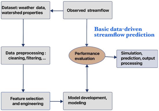
Figure 2.
The fundamental data-driven prediction process.