Your browser does not fully support modern features. Please upgrade for a smoother experience.
Please note this is a comparison between Version 1 by Chaoluo Lv and Version 2 by Jason Zhu.
With the rapid development of wireless communication technology, intelligent communication has become one of the mainstream research directions after the fifth generation (随着无线通信技术的飞速发展,智能通信已成为继第五代(5G). In particular, deep learning has emerged as a significant artificial intelligence technology widely applied in the physical layer of wireless communication for achieving intelligent receiving processing. Channel estimation, a crucial component of physical layer communication, is essential for further information recovery. )之后的主流研究方向之一。特别是,深度学习已成为一种重要的人工智能技术,广泛应用于无线通信的物理层,以实现智能接收处理。信道估计是物理层通信的重要组成部分,对于进一步的信息恢复至关重要。本文旨在综述深度学习方法在信道估计中的应用研究。
- channel estimation
- deep learning
- wireless communication
- physical layer
1. Introduction引言
Deep learning is transforming the paradigms and methods of physical layer communications, with application areas including channel estimation, resource allocation, and signal detection [1][2]. Conventional channel estimation methods work well in systems with a clear and linear representation of the input–output relationship. However, when the wireless environment becomes more complicated, the input–output relationship exhibits nonlinear characteristics, potentially reducing the effectiveness of conventional techniques. Deep learning aims to enable machines to learn to deal with complex and highly nonlinear relationships between input datasets and desired outputs without human intervention [3].
深度学习正在改变物理层通信的范式和方法,其应用领域包括信道估计、资源分配和信号检测[45\u46]。传统的信道估计方法在输入输出关系清晰线性表示的系统中效果很好。然而,当无线环境变得更加复杂时,输入-输出关系表现出非线性特性,这可能会降低传统技术的有效性。深度学习旨在使机器能够在没有人为干预的情况下学习处理输入数据集和期望输出之间复杂且高度非线性的关系[47]。如第1节所述,现有的基于深度学习的信道估计研究大致可分为两大类:数据驱动和模型驱动方法。
2. Neural Networks神经网络
As a branch of artificial intelligence technology, deep learning uses neural networks as models, so it is necessary to briefly introduce neural networks before introducing deep-learning-based channel estimation methods. Neural networks, which mimic the neuronal network of the human brain, consist of input, hidden, and output layers with numerous interconnected neurons through the weights in each layer. By adjusting these weights through learning, neural networks can process input information and produce output. According to the application of deep learning in various fields, the structure of the basic network is different, primarily including the deep neural network (深度学习作为人工智能技术的一个分支,以神经网络为模型,因此在介绍基于深度学习的信道估计方法之前,有必要先简单介绍一下神经网络。神经网络模仿人脑的神经元网络,由输入层、隐藏层和输出层组成,每层的权重都有许多相互连接的神经元。通过学习调整这些权重,神经网络可以处理输入信息并产生输出。根据深度学习在各个领域的应用,基础网络的结构各不相同,主要包括深度神经网络(DNN), convolutional neural network (CNN), recurrent neural network (RNN), generative adversarial network (GAN), etc. Most deep learning models can be combined or optimized based on these four networks. )、卷积神经网络(CNN)、循环神经网络(RNN)、生成对抗网络(GAN)等。大多数深度学习模型都可以基于这四个网络进行组合或优化。
2.1. DNN
A basic structure of DNN is的基本结构如图 shown in Figure 1, which consists of one input layer, 所示,它由一个输入层、L hidden layers, and one output layer, with several neurons in each layer and full个隐藏层和一个输出层组成,每层中有几个神经元,层与层之间完全连接。一个 connectivity between layers. A DNN can be considered a neural network that contains numerous hidden layers, and the purpose of adding multiple hidden layers is to enhance the learning and mapping capabilities of the network. Additionally, to introduce the nonlinearity, activation functions like the sigmoid, rectified linear unit (ReLU), or hyperbolic tangent (Tanh) are applied after the outputs of each layer.DNN 可以被认为是一个包含大量隐藏层的神经网络,添加多个隐藏层的目的是增强网络的学习和映射能力。此外,为了引入非线性,在每层的输出之后应用了 sigmoid、整流线性单元 (ReLU) 或双曲正切 (Tanh) 等激活函数。
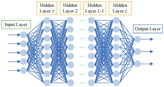
Figure图 1. Basic structure of DNN. 的基本结构。
2.2. CNN美国有线电视新闻网
CNN is among the most representative model structures for deep learning, with the earliest proposition dating back to the publication of the seminal literature [4]. Figure是深度学习最具代表性的模型结构之一,最早的命题可以追溯到开创性文献的发表[48]。图 2 shows a basic显示了一个基本的 CNN structure comprising an input layer, multiple convolutional and pooling layers, a fully connected layer, and an output layer. The input layer’s primary function is to preprocess the data. After this, the convolutional layer extracts features from the processed data, and its output is then mapped nonlinearly via the activation function. Following this, the pooling layer is introduced to decrease computation and prevent overfitting. The convolutional and pooling layers are alternately stacked, and after a series of operations, the output is obtained through the fully connected and output layers. In the convolutional layer, the convolutional kernel is locally connected to its input feature map. For each position in the output feature map, the value is obtained by the weighted sum of the local inputs and connection weights, plus the bias. As this process is equivalent to the convolutional operation, the network is termed a convolutional neural network.结构,包括一个输入层、多个卷积层和池化层、一个全连接层和一个输出层。输入层的主要功能是对数据进行预处理。之后,卷积层从处理后的数据中提取特征,然后通过激活函数对其输出进行非线性映射。在此之后,引入了池化层以减少计算并防止过拟合。卷积层和池化层交替堆叠,经过一系列操作后,通过全连接层和输出层获得输出。在卷积层中,卷积核本地连接到其输入特征图。对于输出特征图中的每个位置,该值由局部输入和连接权重的加权和加上偏差获得。由于该过程等同于卷积运算,因此该网络称为卷积神经网络。
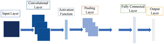
Figure 图2. Basic structure of CNN.的基本结构。
2.3. RNN网络
Figure图 3 shows a显示了一个基本的 basic RNN structure. In contrast to the previously discussed DNN and CNN, RNN is uniquely designed to handle sequential data. It can remember information from past moments and utilize it for the current output calculation. In this case, the nodes among the hidden layers are interconnected. Moreover, the hidden layer’s input depends on both the input layer’s value and the hidden layer’s output from the previous moment.RNN 结构。与前面讨论的 DNN 和 CNN 相比,RNN 专为处理顺序数据而设计。它可以记住过去时刻的信息,并将其用于当前的输出计算。在这种情况下,隐藏层之间的节点是相互连接的。此外,隐藏层的输入取决于输入层的值和隐藏层在前一时刻的输出。
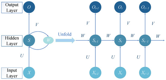
Figure 图3. Basic structure of RNN.的基本结构。
During the training process, 在训练过程中,RNNs may suffer from long-term dependency, leading to gradient vanishing or gradient explosion. Therefore, the literature [5] conducted further research and proposed a special 可能会长期依赖,导致梯度消失或梯度爆炸。因此,文献[49]进行了进一步的研究,并提出了一种特殊的RNN called the long short-term memory (,称为长短期记忆(LSTM) network to effectively resolve this issue.)网络,以有效地解决这一问题。
2.4. GAN氮化镓
Figure图 4 represents表示通用 the general GAN structure, which consists of a generator and a discriminator. The generator receives a latent vector (usually random noise) as input and generates samples analogous to the training data. On the other hand, the discriminator receives samples (which can be real or generated by the generator) as input and predicts their veracity. Notably, the generator and the discriminator train against each other in a competitive and collaborative dynamic. Specifically, the generator’s objective is to trick the discriminator by bringing the generated samples closer and closer to the real samples to the point where they cannot be distinguished accurately. Concurrently, the discriminator is tasked with accurately classifying the samples as possible, thereby heightening the distinction between the real and generated samples. During the iterative adversarial training process, the generator and the discriminator keep adjusting their parameters until they reach an equilibrium point. That is to say, the generator can generate realistic samples, while the discriminator cannot distinguish between real and generated samples.GAN 结构,它由生成器和鉴别器组成。生成器接收潜在向量(通常是随机噪声)作为输入,并生成类似于训练数据的样本。另一方面,鉴别器接收样本(可以是真实的,也可以由生成器生成)作为输入并预测其真实性。值得注意的是,生成器和鉴别器在竞争和协作动态中相互训练。具体来说,生成器的目标是通过使生成的样本越来越接近真实样本,以至于无法准确区分它们来欺骗鉴别器。同时,鉴别器的任务是尽可能准确地对样本进行分类,从而提高真实样本和生成样本之间的区别。在迭代对抗训练过程中,生成器和判别器不断调整其参数,直到达到平衡点。也就是说,生成器可以生成真实的样本,而判别器无法区分真实的样本和生成的样本。
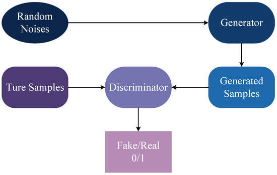
Figure 4. Basic structure of GAN.
3. Toy Example of Deep Learning Application in Channel Estimation
This simulation is set in a vehicular communication scenario within an OFDM system that conforms to the IEEE 802.11p standard. In this environment, the channel exhibits time-varying characteristics, and there is a strong correlation between adjacent OFDM symbols. The classic LS algorithm, performed based on two preambles in an OFDM frame, struggles to track rapid changes in the channel, resulting in poor performance. In contrast, the constructed data pilot (CDP) algorithm constructs virtual pilots from data subcarriers and uses the correlation between adjacent OFDM symbols. It treats the data subcarriers of the previous symbol as a preamble to conduct the current symbol’s channel estimation. This algorithm somewhat improves the channel estimation performance but reduces reliability due to error propagation from one symbol to the next.
Researchers used the VTV Urban Canyon (VTV-UC) channel model with a velocity setting of 48 km/h and a Doppler shift of 500 Hz. To obtain a robust DNN model, researchers trained it at a high SNR of 40 dB. Then, researchers tested it in a SNR range of 0–40 dB and compared its performance with the LS algorithm and the original CDP algorithm. Figure 5a,b display the performance comparison in terms of BER and NMSE, respectively. These results indicate that the DNN-enhanced CDP approach significantly improves the channel estimation accuracy in most scenarios. Even though the performance is not the best in a few low-SNR conditions, it still outperforms the other two traditional algorithms in general, showing the potential of deep learning in channel estimation applications.
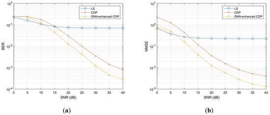
Figure 5. Performance comparison with the LS algorithm and the original CDP algorithm; (a) BER performance comparison; and (b) NMSE performance comparison.
4. Data-Driven Deep-Learning-Based Channel Estimation Methods
Figure 6 illustrates the structure of a simple channel estimator based on data-driven deep learning. The core idea of the data-driven approach is to consider neural networks as “black boxes”, replacing the original traditional communication system structure with them and perpetually updating their parameters through training with massive amounts of data.
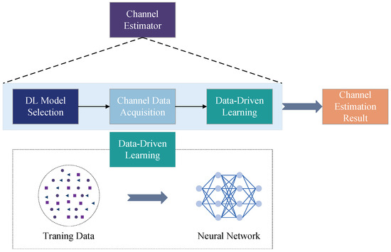
Figure 6. Structure of a data-driven deep-learning-based channel estimator.
4.1. Application of DNN in Data-Driven Channel Estimation
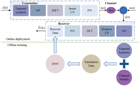
DNN is a fundamental network for deep learning with a simple model, and as such, it was first applied in channel estimation. It allows end-to-end learning, i.e., from the original input to the target output. Figure 7 shows a DNN-based channel estimator proposed in [6][9], serving as one of the typical examples. In this model, the authors estimated the CSI end-to-end by recovering the transmitted data from the received data, including the pilot and data blocks. Moreover, DNN is highly adaptable and flexible, and its structure and hyperparameters can be modified to accommodate various application scenarios.
In 2020, Ma et al. [7][51] investigated a DNN-based method that combines channel estimation and pilot design. The proposed DNN model is composed of a dimensionality reduction subnetwork and a reconstruction subnetwork. In the first subnetwork, the fully connected layer is designed to compress the high-dimensional channel vector into low-dimensional received measurements, and this compression process treats the weights in the layer as pilot signals. In the second subnetwork, several cascaded convolutional layers and a fully connected layer are designed to recover the high-dimensional channel. Through experimental comparison, this method exhibits a superior NMSE performance to the simultaneous orthogonal matching pursuit (SOMP) algorithm. Furthermore, when the DNN trained with multi-carrier samples is tested on single-carrier samples, and it still performs well, demonstrating its excellent generalization ability.
The interpolation approach is closely connected with the performance of the pilot-based method. In [8][52], Ge et al. proposed to utilize DNN to replace the interpolation process of the conventional pilot-based method. Firstly, the position index and the channel estimation result of pilot subcarriers are used as training data to train the DNN model. Then, the position index of data subcarriers is used as the input to the DNN, and the channel estimation of data subcarriers is finally obtained. This method does not require prior statistics or matrix inverse operations like the MMSE algorithm and thus has a lower complexity. Moreover, the proposed method exhibited superior estimation accuracy in experiments compared to the LS algorithm, which requires interpolation. Finally, the author tested the model trained with eight multipath paths in conditions with 4, 8, and 12 multipath paths. The BER performance remains almost unchanged, showing the excellent generalization ability of the proposed model.
In 2021, Zheng et al. [9][53] developed an online DNN-based channel estimation method under limited pilot conditions. This method can dynamically learn and compute in real time, inferring and updating the DNN weights from the pilot symbols received online without knowing the real channel matrix to adapt to the actual communication environment. The proposed DNN-based method exhibits the strongest robustness in experiments. Furthermore, its estimation accuracy approaches the group orthogonal matching pursuit (GOMP) algorithm and the burst LASSO algorithm while surpassing the MMSE algorithm. Significantly, it surpasses all these methods by orders of magnitude in terms of computational speed. Additionally, the proposed DNN model, trained at an SNR of 30 dB, consistently surpasses the MMSE algorithm in terms of NMSE performance when tested at lower SNR levels. Specifically, the experiments conducted on the 3GPP SCM TR 25.996 and the DeepMIMO channel models can both yield this result, demonstrating the model’s strong generalization on lower SNR.
In the realm of ocean exploration, underwater acoustic (UWA) communication is pivotal. In 2022, Zhang et al. [10][54] investigated a DNN-based scheme for underwater acoustic channel estimation in OFDM systems. The DNN utilizes transmitted pilots and received symbols in this scheme to reconstruct the UWA channel. Encouragingly, the scheme shows outstanding signal detection performance on the estimated channel. Simulation results demonstrate its efficacy, reducing the BER by over 40% in comparison to the LS algorithm. Furthermore, as the pilot number grows, the BER performance approaches that of the MMSE algorithm.
To improve the estimation performance in impulse noise environments, Li et al. [11][55] developed a method based on the denoising autoencoder-DNN (DAE-DNN). The proposed method consists of three steps: first, utilizing DAE for preprocessing, namely learning the impaired data and restoring clean received signals under conditions where impulse noise is present; second, employing the preprocessed data from DAE to train the DNN offline; and finally, the DNN estimates the CSI online. Experimental results demonstrate that this method has strong robustness under impulse noise conditions, outperforming the MMSE algorithm, the orthogonal matching pursuit (OMP) algorithm, and the LS algorithm in terms of MSE and BER.
4.2. Application of CNN in Data-Driven Channel Estimation
CNN is advantageous for channel estimation since it can reduce the computation of feature parameters and automatically select the appropriate training weights. In addition, CNN’s excellent feature extraction capability contributes to its excellent image processing performance. Hence, the channel estimation problem can be transformed into an image processing problem in the application, enabling it to learn from the training data and obtain accurate CSI. Figure 8 shows examples of transforming the channel time–frequency response into a 2D image under the Vehicular-A (VehA) channel model [12][56]. Specifically, Figure 8a,b represent the channel time–frequency response images under the perfect channel model without noise and the noisy channel model with an SNR of 22 dB, respectively.
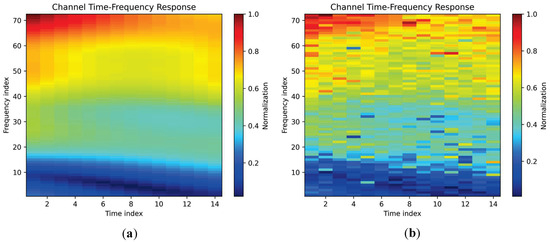
Figure 8. Two-dimensional image examples of the channel time–frequency response: (a) under the VehA perfect channel model (without noise); and (b) under the VehA noisy channel model (SNR = 22 dB).
In 2019, the ChannelNet proposed by Soltani et al. [13][57] with regard to the channel time–frequency response as a low-resolution 2D image and the values are only known at pilot positions. The ChannelNet consists of a super-resolution CNN (SRCNN) and a denoising CNN (DnCNN), which are cascaded into a two-step channel estimator. In the first step, the low-resolution image is enhanced into a high-resolution image by the SRCNN. In the second step, the DnCNN removes the noise effect to obtain a higher-quality image (i.e., an accurately estimated channel). Through experimental verification, the ChannelNet’s MSE performance is superior to the ALMMSE algorithm (an approximation to linear MMSE) but inferior to the MMSE algorithm in low SNR. However, the performance of ChannelNet trained at the SNR of 22 dB shows a decreasing trend when the SNR exceeds 23 dB, which indicates that its generalization ability on real noise is not good enough. Notably, this literature is a pioneer in using image processing methods for channel estimation, providing a novel idea for many subsequent studies. Inspired by this, Li et al. [14][58] investigated a deep residual channel estimation network (ReEsNet) based on residual learning, which can work in a wide range of scenarios and significantly reduce the complexity while improving estimation accuracy.
The numerous convolutional layers in the denoising structure (DnCNN) of ChannelNet [13][57] lead to a large amount of computation and a long execution time, which greatly consumes memory. For this reason, Pradhan et al. [15][59] made improvements and proposed the channel estimation network (CENet). Compared with ChannelNet, CENet also uses SRCNN for image resolution enhancement, with the difference that a convolutional blind denoising network (CBDNet) is used as the denoising structure instead of DnCNN. The CBDNet reduces the overall number of convolutional layers, thereby reducing the complexity of the proposed CNN model. Through experimental comparison, the CENet is superior to the ChannelNet but inferior to the ideal MMSE algorithm in terms of MSE. Furthermore, the author tested the CENet trained with 48 pilots under conditions of different numbers of pilots. The results showed that CENet maintains high performance even with fewer pilots, unlike other methods, which exhibited a significant decrease in performance under the same conditions.
Most research utilizing deep learning for channel estimation focuses on constructing complex neural networks, which leads to increased storage and computational requirements. Li et al. [16][60] addressed this phenomenon by combining the CNN and Transformer and proposing a lightweight channel estimation Transformer (LCET). This scheme treats the channel response matrix as a 2D image, with the channel features extracted using a lightweight feature extraction CNN (LFEC) and then transmitted to a lightweight-adjusted Transformer (LAT) for channel estimation. Through experimental comparison, the estimation accuracy of the LCET surpasses the LS algorithm and some neural networks, closely approximating the performance of LMMSE algorithms in multi-pilot scenarios.
In general, the transceiver of millimeter wave (mmWave) massive MIMO systems employs a hybrid precoding structure, and thus, the acquisition of CSI in the low SNR regime poses difficulties. To overcome this challenge, Zhao et al. [17][61] proposed ResNet-UNet, a network that combines the residual network (ResNet) and the U-shaped network (U-Net) for channel estimation. In particular, the proposed ResU-net consists of a denoiser and an estimator. Firstly, the received noisy pilot signal is converted into an image and processed by the denoiser. Then, the obtained clean pilot signal image is fed to the estimator to obtain the estimation result. Through experimental verification, the Res-UNet surpasses the conventional algorithms and the deep CNN in estimation accuracy and is robust to noisy environments.
In 2023, Rahman et al. [18][62] proposed a deep residual convolutional blind denoising network (ResCBDNet) for massive MIMO visible light communication systems to estimate more realistic and accurate CSI. The proposed ResCBDNet comprises two subnetworks: the noise estimation network and the non-blind denoising network, and it transforms the sparse channel matrix into a 2D image. Initially, the scheme employs a noise estimation network to enhance the generalization ability of the true noise. It then interactively reduces the effect of noise in the channel matrix through the adjustment of the noise level mapping. Subsequently, the noiseless estimated channel is recovered using the non-blind denoising network. Experiments demonstrate that the ResCBDnet surpasses some existing deep-learning-based methods in terms of normalized MSE (NMSE) and peak SNR (PSNR). Moreover, with its exceptional noise generalization capability, ResCBDNet demonstrates the superior MSE performance to other methods when SNR = 20 dB.
4.3. Application of RNN in Data-Driven Channel Estimation
RNN is not as widely used as other neural networks in channel estimation. However, some researchers have recently delved into RNN-based methods to improve the channel estimation accuracy. Given the time-dependent properties of RNN, it can be used for time-varying channels to improve time-series information processing. Moreover, it is especially well suited for channel estimation in high-speed mobile settings.
For high-speed mobile environments, channel estimation becomes problematic due to the impact of multipath and Doppler effects, and conventional methods perform poorly due to the limited number of available pilots. Consequently, Gizzini et al. [19][63] proposed a frame-by-frame (FBF) channel estimation method based on bi-directional RNN (Bi-RNN) for doubly-selective channels. The goal is to perform end-to-end 2D interpolation after estimating the channel of pilot symbols, thereby obtaining the channel estimation of data symbols. Simulation results demonstrate that the proposed Bi-RNN is robust and adaptive, and the estimation accuracy is superior to some existing deep learning schemes. Although the estimation accuracy is marginally lower than the conventional 2D-LMMSE algorithm, the complexity is reduced by nearly 106
times, making it a viable alternative.
In 2021, Essai Ali et al. [20][64] estimated CSI using a variant of LSTM, namely a bi-directional LSTM (Bi-LSTM) neural network. The proposed network model relies on pilot assistance, does not require prior knowledge of channel statistical information, and employs online training with offline deployment. Under the conditions of limited pilots and uncertain channel prior statistics, this model is robust and has a superior symbol error rate (SER) performance over the LSTM and the conventional algorithms (LS and MMSE). The proposed Bi-LSTM can analyze massive data and establish relationships between features, thus having excellent generalization capabilities and applicability to new datasets.
The gated recurrent unit (GRU) is a lightweight variant with potential developed from LSTM. In 2022, Essai Ali et al. [21][65] designed an end-to-end channel estimation method based on GRU to recover the transmitted signal from the received signal, thereby estimating the CSI. Through experimental verification, the GRU-based method surpasses the conventional estimation algorithms (LS and MMSE), DNN, and ReEsNet in terms of SER. In 2023, Helmy et al. [22][66] combined LSTM and GRU to develop an LSTM-GRU estimator, which is designed for channel estimation from the received signal. It consists of three parts: the LSTM, the GRU, and the smoothing module. In this framework, the LSTM serves as a minimum absolute filter that denoises the pre-processed received signals, and the GRU module compensates for the information loss in the LSTM module as a compensator. Finally, the model’s output is smoothed using batch normalization and convolutional layers. Through experimental comparison, the proposed LSTM-GRU estimator has a superior NMSE performance over the CNN and CGAN estimators. Additionally, the LSTM-GRU trained with a pilot length of 8 is tested in scenarios of varying pilot lengths. The estimation performance of this model does not degrade significantly in the short pilot length range, indicating its outstanding generalization ability.
4.4. Application of GAN in Data-Driven Channel Estimation
In channel estimation, GAN has the ability to serve by generating additional data to augment the required training dataset, which is particularly valuable in scenarios without sufficient information about the actual CSI. Moreover, GAN can adaptively improve its performance during training, thereby achieving more accurate estimation results through the adversarial process between the generator and the discriminator.
Motivated by ReEsNet in [14][58], Zhao et al. [23][67] developed a super-resolution GAN (SRGAN) for channel estimation in 2021. However, the estimation results of ReEsNet have lost high-frequency details and failed to match the desired fidelity at higher resolutions. In the SRGAN scheme, the channel generated by the generator is closer to the actual channel distribution. Meanwhile, the discriminator recovers more details, significantly enhancing the estimation accuracy. Through experimental comparison, the SRGAN’s MSE performance surpasses both the LS algorithm and the ReEsNet, and it approaches the MMSE algorithm in high SNR.
For massive MIMO systems, Dong et al. [24][68] investigated a CGAN channel estimator in the same year. The proposed CGAN learns how to map from quantized observations to the actual channel and learns a suitable adaptive loss function for network training, resulting in a highly robust model and a more realistic estimated channel. Even when the model is tested on a different channel (i.e., a millimeter wave channel), its performance remains almost unchanged, demonstrating its exceptional generalization capability. In 2023, Zhang et al. [25][69] also employed CGAN, but their focus was obtaining accurate CSI for MIMO-OFDM systems in high-speed railway scenarios. Their scheme is executed in two steps and regards the pilot signal as a 2D image. In the denoising step that employs the U-Net framework, the received noisy pilot image is denoised using the Noise2Noise (N2N) algorithm. In the estimation step, the CGAN completes the channel estimation by learning the features of the denoised pilot image. Through experimental verification, the N2N-CGAN has high estimation accuracy in high-speed mobile scenarios, exhibits strong robustness in noisy environments, and has low computational complexity.
In the pilot-based channel estimation scheme, the estimation efficacy highly depends on the pilot insertion pattern. To improve the estimation accuracy while reducing the pilot overhead, Kang et al. [26][70] proposed a network model called CAGAN as a channel estimation scheme for joint pilot design. The CAGAN comprises a CGAN and a concrete autoencoder (concrete AE). First, the concrete AE is used to search for the most informative location in the time–frequency grid and insert pilots here, thereby optimizing the pilot design. Next, the optimized pilots are fed into the CGAN for channel estimation. Experimental results show that the CGAN can exhibit outstanding estimation performance with a limited number of pilots. In order to verify the generalization ability of noise, the CAGANs trained with an SNR of 15 dB and trained at different SNRs are compared in a 0–30 dB SNR range. The result demonstrates that, when the SNR is above 9 dB, the performance of these two models is comparable.
5. Model-Driven Deep-Learning-Based Channel Estimation Methods
The model-driven approach is built on known mathematical models, and its central idea is to combine deep learning with conventional algorithms to improve or expand existing methods. Moreover, it does not depend on extensive labeled data to select the right standard neural network, thus making deep learning more interpretable and predictable. Figure 9 illustrates the components of the model-driven approach. Currently, most research on model-driven channel estimation primarily unfolds on the basis of the LS algorithm and the algorithms in compressive sensing (CS) that include the OMP algorithm and the approximate message passing (AMP) algorithm.
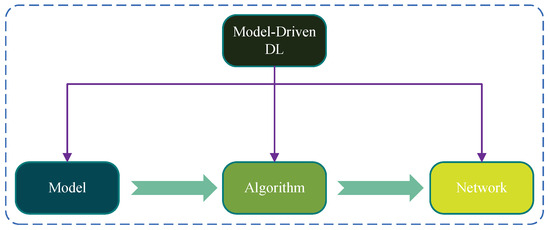
Figure 9. Components of the model-driven approach.
4.1. Model-Driven Channel Estimation Combining LS Algorithm
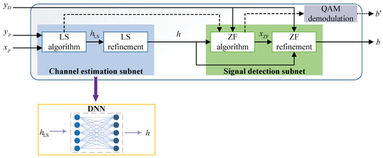
As previously mentioned, the conventional LS channel estimation algorithm is computationally simple but leads to poor performance since it ignores the impact of noise. The ComNet proposed by Gao et al. [27][12] solves the problem using deep learning networks, which provides a reference for subsequent research. As shown in Figure 10, the ComNet is constructed by cascading the channel estimation and the signal detection subnets. In the channel estimation subnet part, the authors utilized a DNN to refine the coarse estimation of the traditional LS algorithm. Specifically, the DNN takes the LS coarse estimation as input and learns from the discrepancies between this initial estimation and the actual channel. Then, the DNN adjusts its parameters through training to minimize the prediction error, resulting in a more accurate channel estimation.
In 2021, Jiang et al. [28][71] introduced a dual CNN structure to improve the LS algorithm’s estimation accuracy with lower complexity than the general CNN-based methods. The initial channel estimation obtained by the LS algorithm is used as the input for the dual CNN, which consists of a spatial-frequency CNN (SFCNN) and an angle-delay CNN (ADCNN). In particular, the SFCNN effectively leverages the channel’s sparsity to process white noise, while the ADCNN utilizes the channel correlation to reduce interference. These two CNNs are connected through a discrete Fourier transform (DFT) process. Owing to the dual CNN combining the advantages of SFCNN and ADCNN, it exhibits superior NMSE performance to the single-domain CNN in experiments.
In 2023, Haq et al. [29][72] innovatively implemented channel estimation on a System on Chip (SoC) based on deep learning. Specifically, the authors proposed a channel estimation method called DNN-augmented LS (LSDNN) for the preamble-based OFDM physical layer. This method employs a fully connected feedforward DNN to process the LS estimation results. Specifically, the DNN uses the initial LS estimation as input, learning from its errors to improve the initial estimation. It does this by minimizing the cost function, thereby refining the LS estimation of the previous preamble. Finally, the proposed LSDNN, the LS algorithm, and the LMMSE algorithm are mapped onto a Zynq multiprocessor SoC (ZMPSoC) platform for extensive experimental comparison. Experimental results verify that the LSDNN has a superior estimation accuracy over the LS and the LMMSE algorithms. However, there is still room for improvement in resource utilization and power consumption.
To overcome the challenge of SNR mismatch in multipath time-varying channels, Li et al. [30][73] introduced a cascaded network called NDR-Net for channel estimation. The NDR-Net consists of a cascade of a noise level estimation subnet (NLE), a DnCNN, and residual learning, and the channel matrix is regarded as an image in this scheme. Firstly, the LS algorithm estimates the coarse value of the channel matrix, which is then inputted into NLE to obtain the noise level estimation. Subsequently, the estimated noise level and the initial noisy channel matrix image are inputted into DnCNN for noise reduction, resulting in a pure noisy image. Finally, the noiseless channel matrix image is obtained by residual learning. Through experimental comparison, the NDR-Net has better estimation accuracy than conventional methods when the SNR is mismatched. In addition, it applies to different Doppler shifts.
4.2. Model-Driven Channel Estimation Combining OMP Algorithm
As a greedy algorithm, the OMP algorithm offers optimal solutions to sparse recovery problems. Leveraging the sparsity of channels, it facilitates channel estimation with minimized pilot overhead. However, due to the grid mismatch issue, the OMP algorithm may not provide satisfactory estimation results [31][74]. To achieve better channel estimation performance, combining the OMP algorithm with deep learning is a viable approach.
In 2022, Li et al. [32][75] designed a model-driven ResNet-based scheme for orthogonal time–frequency space (OTFS) systems. Considering the sparsity of the channel in the delay-Doppler domain, they first employed the OMP algorithm to obtain a coarse estimation. Then, this initial estimation was fed into the proposed ResNet for a more accurate result. During the training process, the ResNet learns from the error between the OMP rough estimation and the actual channel response. Then, this network continuously optimizes the parameters, resulting in a more realistic channel estimation result. Compared to the conventional OMP algorithm, the ResNet-based scheme has a superior NMSE performance. Furthermore, it applies to various scenarios and displays outstanding robustness to Doppler spread.
In [33][76], Tong et al. introduced a two-step OMP-based channel estimation algorithm. First, a composite convolution kernel function (CKF) is constructed based on the autocorrelation matrix, which then coarsely estimates the angles of arrival/departure (AoAs/AoDs) for multipath channels. Second, a squeeze-and-excitation ResNet (SE-ResNet) utilizing the Noise2Void (N2V) algorithm is proposed to refine the AoAs/AoDs estimation. Then, the channel amplitude is estimated using the LS algorithm. Finally, the channel matrix is accurately recovered based on all the results above. In the experiments, the proposed algorithm exhibits a superior NMSE performance over the simultaneous weighted OMP (SW-OMP) algorithm, the Newtonized OMP (NOMP) algorithm, and the channel estimation neural network (CENN), while having computational complexity.
To enhance the effectiveness of the conventional OMP algorithm in hybrid-field channel estimation, Nayir et al. [34][77] developed a novel scheme called OMP-CAE by incorporating the convolutional autoencoder (CAE) for massive MIMO channels. In this scheme, the OMP algorithm first provides a rough channel estimation. Since the channel parameters from the OMP rough estimation contain significant errors at low SNR, they are fed into the CAE network. Then, the CAE network uses its strong denoising ability to improve the accuracy of channel estimation. Through experimental verification, the OMP-CAE surpasses the MMSE algorithm and the conventional OMP algorithm in terms of NMSE and applies to different scenarios.
4.3. Model-Driven Channel Estimation Combining AMP Algorithm
The AMP algorithm is a significant iterative algorithm that excels at recovering sparse signals. It can achieve channel estimation in sparse channel environments with low computational complexity [35][78]. Nevertheless, the AMP algorithm’s performance is highly dependent on certain preset parameters, and it presents a challenge to determine the optimal parameters, leading to its limited estimation performance. Therefore, some researchers have combined the AMP algorithm with deep learning. This approach allows the deep learning network to learn and optimize the iterative steps of the AMP algorithm, forming a novel and effective channel estimation method.
The learned AMP (LAMP) algorithm is a variant of the AMP algorithm that unfolds and maps the AMP algorithm’s iterative steps directly into a DNN, thereby utilizing the DNN’s ability to jointly optimize the coefficients of the linear transformations and the parameters of the nonlinear shrinkage function. However, the existing LAMP networks may not achieve the desired performance in beamspace channel estimation. In light of this, Wei et al. [36][79] investigated an enhanced scheme based on a prior-assisted Gaussian mixture LAMP (GM-LAMP). Specifically, the authors replaced the soft threshold shrinkage function in the original LAMP network with a Gaussian mixture shrinkage function, which is able to reflect more of the beamspace channel’s prior information. Compared to the OMP, the AMP, and the LAMP algorithms, the GM-LAMP algorithm has a superior NMSE performance with less pilot overhead.
The denoising AMP (DAMP) algorithm is also a variant stemming from the AMP algorithm, replacing the shrinkage function with a denoiser. Pu et al. [37][80] deeply unfolded the DAMP algorithm by replacing its original denoiser with a DnCNN. They developed the model-driven learned denoising AMP (LDAMP) algorithm for channel estimation with noisy channels in OTFS systems. Then, they predicted the theoretical NMSE performance of the LDAMP algorithm using the state evolution (SE) equation. Owing to the integration of the DAMP algorithm’s superior performance and the nonlinear fitting capability of deep learning, the proposed algorithm exhibits effectiveness and high accuracy.
In 2022, Wang et al. [38][81] introduced an AMP-based multi-stage scheme with deep learning for quasi-sparse channel environments. This scheme treats the entire system as an end-to-end DNN, and each iterative process of the sensing matrix, noise introduction, and AMP algorithm is regarded as a DNN layer. Firstly, the AMP sensing matrix is trained to adapt to the quasi-sparse channel and learn the optimal sensing matrix. Secondly, the AMP algorithm’s nonlinear shrinkage parameters and linear coefficients are optimized layer-by-layer. Finally, all trainable parameters are jointly optimized, thereby optimizing the entire system. Compared to the AMP, the LAMP, and the LDAMP algorithms, the proposed scheme has a superior NMSE performance while reducing pilot overhead.
Nevertheless, the studies mentioned above are limited to traditional communication scenarios and do not address future communication scenarios. As one of the critical techniques for 6G networks, the research on RIS is in full swing. The introduction of RIS improves the performance of communication systems but also increases their complexity, making conventional techniques, including channel estimation, confront new challenges. With the accelerated advancement in deep learning, numerous researchers have adopted this technique to solve the aforementioned issue. The following section will introduce channel estimation methods based on deep learning for RIS-aided wireless communication systems.