Your browser does not fully support modern features. Please upgrade for a smoother experience.
Please note this is a comparison between Version 1 by Georgios Fotis and Version 2 by Peter Tang.
Precise anticipation of electrical demand holds crucial importance for the optimal operation of power systems and the effective management of energy markets within the domain of energy planning. The primary aim of bidirectional Long Short-Term Memory (LSTM) network is to enhance predictive performance by capturing intricate temporal patterns and interdependencies within time series data.
- forecasting electricity demand
- bidirectional LSTM
- short-term prediction
- medium-term prediction
1. Introduction
A vital area of research within the field of power systems is that of electric load forecasting (ELF), owing to its pivotal role in system operation planning and the escalating scholarly attention, it has attracted [1]. The precise prediction of demand factors, encompassing metrics like hourly load, peak load, and aggregate energy consumption, stands as a critical prerequisite for the efficient governance and strategizing of power systems. The categorization of ELF into three distinct groups, as shown below, caters to diverse application requisites:
-
Long-term forecasting (LTF): Encompassing a time frame of 1 to 20 years, LTF plays a pivotal part in assimilating new-generation units into the system and cultivating transmission infrastructure.
-
Medium-term forecasting (MTF): Encompassing the span of 1 week to 12 months, MTF assumes a central role in determining tariffs, orchestrating system maintenance, financial administration, and harmonizing fuel supply.
-
Short-term forecasting (STF): Encompassing the temporal span of 1 h to 1 week, STF holds fundamental significance in scheduling the initiation and cessation times of generation units, preparing spinning reserves, dissecting constraints within the transmission system, and evaluating the security of the power system.
Distinct forecasting methodologies are employed corresponding to the temporal horizon. While MTF and LTF forecasting often hinge upon trend analysis [2][3][2,3], end-use analysis [4], NN techniques [5][6][7][5,6,7], and multiple linear regressions [8], STF necessitates approaches such as regression [9], time series analysis [10], artificial NNs [11][12][13][14][11,12,13,14], expert systems [15], fuzzy logic [16][17][16,17], and support vector machines [18][19][18,19]. STF emerges as particularly critical for both transmission system operators (TSOs), guaranteeing the reliability of system operations during adverse weather conditions [20][21][20,21], and distribution system operators (DSOs), given the increasing impact of microgrids on aggregate load [22][23][22,23], along with the challenge of assimilating variable renewable energy sources to meet demand. Proficiency in data analysis and a profound comprehension of power systems and deregulated markets are prerequisites for successful performance in MTF and LTF, STF primarily emphasizes the use of data modeling to match data with suitable models, rather than necessitating an extensive understanding of power system operations [24]. Accurate daily-ahead load forecasts (STF) stand as imperative for the operational planning department of every TSO year-round. The precision of these forecasts dictates which units partake in energy generation to satisfy the system’s load requisites the subsequent day. Several factors, including load patterns, weather circumstances, air temperature, wind speed, calendar information, economic occurrences, and geographical elements, have an impact on load forecasting [25]. Prudent load projections profoundly influence strategic decisions undertaken by entities such as power generation companies, retailers, and aggregators, given the deregulated and competitive milieu of modern power markets. Furthermore, resilient predictive models offer advantages to prosumers, assisting in the enhancement of resource management, encompassing energy generation, control, and storage. Nonetheless, the rise of “active consumers” [26] and the increasing integration of renewable energy sources (RES) from 2029 to 2049 [27] will bring about novel planning and operational complexities (Commission, 2020). As uncertainties stem from RES energy outputs and power consumption, sophisticated forecasting techniques [28][29][30][28,29,30] become imperative. Consequently, a deep learning (DL) forecasting model was innovated to assess and predict the future of electricity consumption, with the intent of mitigating potential power crises and harnessing opportunities in the evolving energy landscape.
Electrical load prediction has evolved into a critical research field due to the rising demand for effective energy management and resource allocation. Numerous machine learning techniques have been employed in this domain, encompassing traditional time series methods [10], neural and deep learning models [11][12][11,12]. Among these methods, bidirectional LSTM (biLSTM) networks have emerged as a prominent and promising approach for achieving accurate and robust electrical load prediction.
2. LSTM Networks
In 1997, Hochreiter and Schmidhuber introduced LSTM networks [31] as a specialized variant of RNNs tailored to effectively manage and learn from long-term dependencies in data. Their pervasive adoption and demonstrated success across a range of problem domains have propelled LSTMs into heightened prominence. Unlike traditional RNNs, LSTMs are explicitly engineered to tackle the challenge of prolonged dependencies, constituting an innate feature of their functioning. LSTMs are constructed from a sequence of recurrent modules, a common trait shared with all RNNs. Yet, it is the configuration of these repeating modules that sets LSTMs apart. In contrast to a solitary layer, LSTMs encompass four interconnected layers. The pivotal distinction within LSTMs arises from the incorporation of a cell state—a horizontal conduit running through the modules that orchestrate seamless information propagation. The transmission of data within the cell state is governed by gates, which comprise a neural network layer based on the sigmoid function connected with a pointwise multiplication operation. The sigmoid layer generates values in the range of 0 to 1, dictating the extent of the passage of information. The fundamental architecture of the LSTM model is visually depicted in Figure 1.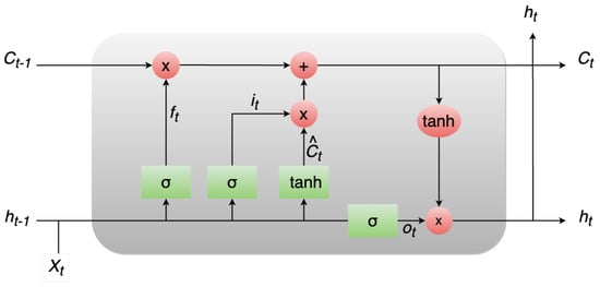
Figure 1.
The LSTM model architecture.
3. BiLSTM
The BiLSTM network [32] constitutes a sophisticated variant of the LSTM architecture. LSTM, in itself, is a specialized form of Recurrent Neural Network (RNN) that has been proven effective in handling sequential data, such as text, speech, and time-series data. However, standard LSTM models have limitations when it comes to capturing bidirectional dependencies within the data, which is where BiLSTM steps in to overcome this constraint. At its core, the BiLSTM network introduces bidirectionality by processing input sequences both forward and backward through two separate LSTM layers. By doing so, the model can exploit context from past and future information simultaneously, leading to a more comprehensive understanding of the data. This distinctive competence renders it especially apt for endeavors necessitating a profound examination of sequential patterns, such as sentiment analysis, named entity recognition, machine translation, and related tasks. The key advantages of bidirectional LSTMs are:-
Enhanced Contextual Understanding: By considering both past and future information, bidirectional LSTMs better understand the context surrounding each time step in a sequence. This is particularly useful for tasks where the meaning of a word or a data point is influenced by its surrounding elements.
-
Long-Range Dependencies: Bidirectional LSTMs can capture long-range dependencies more effectively than unidirectional LSTMs. Information from the future can provide valuable insights into the context of earlier parts of the sequence.
-
Improved Performance: In tasks like sequence labeling, sentiment analysis, and machine translation, bidirectional LSTMs often outperform unidirectional LSTMs because they can better capture nuanced relationships between elements in a sequence.
-
Computational Complexity: Since bidirectional LSTMs process data in two directions, they are computationally more intensive than their unidirectional counterparts. This can result in extended training durations and elevated memory demands.
-
Real-Time Applications: In real-time applications where future information is not available, bidirectional LSTMs might not be suitable, as they inherently use both past and future context.
-
Causal Relationships: Bidirectional LSTMs may introduce possible causality violations when used in scenarios where future information is not realistically available at present.
-
Input Layer: The input layer is the first step in the BiLSTM network and serves as the entry point for sequential data. It accepts the input sequence, which could be a sequence of words in natural language processing tasks or time-series data in other applications. The data is typically encoded using word embeddings or other numerical representations to enable the network to process it effectively. The input layer bears the responsibility of transforming the unprocessed input into a structure comprehensible by subsequent layers.
-
LSTM Layers (Forward and Backward): The fundamental element of the BiLSTM network is composed of two LSTM layers: one dedicated to sequentially processing the input sequence in a forward manner, while the other focuses on processing it in a reverse direction. These LSTM layers play a pivotal role in capturing temporal correlations and extensive contextual information embedded within the data. In the forward LSTM layer, the input sequence is systematically processed from the sequence’s initiation to its conclusion, whereas in the backward LSTM layer, the sequence is processed in a reverse manner. By encompassing dual-directional data processing, the BiLSTM effectively captures insights from both historical and prospective facets of the input, enabling adept modeling of bidirectional relationships. Each LSTM cell situated within these layers incorporates a set of gating mechanisms—namely, input, output, and forget gates—that meticulously govern the course of information flow within the cell. This orchestration ensures the network’s retention of crucial information over extended temporal spans, thereby mitigating the issue of vanishing gradients and substantially enhancing gradient propagation during the training phase.
-
Merging/Activation Layer: Following the sequential processing by the forward and backward LSTM layers, the fusion layer takes center stage. The principal aim of this layer is to seamlessly amalgamate the insights garnered from both directions. This amalgamation is typically accomplished by concatenating the hidden states of the forward and backward LSTMs at each discrete time step. This concatenated representation thus encapsulates knowledge encompassing both anterior and forthcoming contexts for every constituent within the input sequence. This amalgamated representation serves as the fundamental bedrock upon which the ensuing layers base their informed decisions, enriched by bidirectional context.
-
Output Layer: Serving as the ultimate stage within the BiLSTM network, the outcome generation layer undertakes the task of processing the concatenated representation obtained from the fusion layer to yield the intended output. The design of the outcome generation layer depends on the specific objective customized for the BiLSTM. For example, in sentiment analysis, this layer might comprise a solitary node featuring a sigmoid activation function to predict sentiment polarity (positive or negative). In alternative applications like machine translation, the outcome layer could encompass a softmax activation function aimed at predicting the probability distribution of target words within the translation sequence. The outcome layer assumes the responsibility of mapping the bidirectional context, assimilated by the BiLSTM, into the conclusive predictions or representations that align with the precise objectives of the designated task.
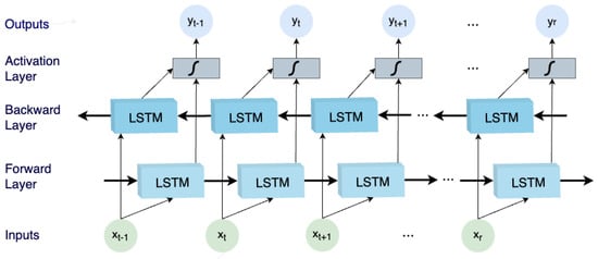
Figure 2.
The BiLSTM basic architecture.