Machine Learning Techniques for Customer Churn Prediction

Machine Learning Techniques for Customer Churn Prediction: Comparison

Please note this is a comparison between Version 1 by Mehdi Imani and Version 4 by Fanny Huang.

This pape r explores the application of various machine learning techniques for predicting customer churn in the telecommunications sector is explored. Researchers. We utilized a publicly accessible dataset and implemented several models, including Artificial Neural Networks, Decision Trees, Support Vector Machines, Random Forests, Logistic Regression, and gradient boosting techniques (XGBoost, LightGBM, and CatBoost). To mitigate the challenges posed by imbalanced datasets, researcherswe adopted different data sampling strategies, namely SMOTE, SMOTE combined with Tomek Links, and SMOTE combined with Edited Nearest Neighbors. Moreover, hyperparameter tuning was employed to enhance model performance. Resarchers'Our evaluation employed standard metrics, such as Precision, Recall, F1-score, and the Receiver Operating Characteristic Area Under Curve (ROC AUC). In terms of the F1-score metric, CatBoost demonstrates superior performance compared to other machine learning models, achieving an outstanding 93% following the application of Optuna hyperparameter optimization. In the context of the ROC AUC metric, both XGBoost and CatBoost exhibit exceptional performance, recording remarkable scores of 91%. This achievement for XGBoost is attained after implementing a combination of SMOTE with Tomek Links, while CatBoost reaches this level of performance after the application of Optuna hyperparameter optimization.

machine learning
churn prediction
SMOTE
imbalanced data
hyperparameter optimization
Optuna
Boosting techniques
Bagging techniques
classification methods
ensemble techniques

1. Introduction

The implementation of Customer Relationship Management (CRM) is a strategic approach to managing and enhancing relationships between businesses and their customers. CRM is a tool employed to gain deeper insights into the requirements and behaviors of consumers, specifically end users, with the aim of fostering a more robust and meaningful relationship with them. Through the utilization of CRM, businesses can establish an infrastructure that fosters long-term and loyal customers. This concept is relevant across various industries, such as banking ^[1][2][3][4][1,2,3,4], insurance companies [5], and telecommunications ^{[6][7][8][9][10][11][12][13][14]}[6,7,8,9,10,11,12,13,14], to name a few.

The telecommunications sector assumes a prominent role as a leading industry in revenue generation and a crucial driver of socioeconomic advancement in numerous countries globally. It is estimated that this sector incurs expenditures of approximately 4.7 trillion dollars annually ^[1][2][1,2]. Within the sector, there exists a high degree of competition among companies, driven by their pursuit of augmenting revenue streams and expanding the market influence through the acquisition of an expanded customer base. A key objective of CRM is customer retention, as studies have demonstrated that the cost of acquiring new customers can be 20 times higher than retaining existing ones [1]. Therefore, maintaining existing customers in the telecommunications industry is crucial for increasing revenue and reducing marketing and advertising costs.

The telecommunications sector is grappling with the substantial issue of customer attrition, commonly referred to as churn. This escalating issue has prompted service providers to shift their emphasis from acquiring new customers to retaining existing ones, considering the significant costs associated with customer acquisition. In recent years, service providers have been progressively emphasizing the establishment of enduring relationships with their customers. Consequently, these providers uphold CRM databases wherein every customer-specific interaction is systematically documented [5]. CRM databases serve as valuable resources for proactively predicting and addressing customer requirements by leveraging a combination of business processes and machine learning (ML) methodologies to analyze and understand customer behavior.

The primary goal of ML models is to predict and categorize customers into one of two groups: churn or non-churn, representing a binary classification problem. As a result, it is imperative for businesses to develop practical tools to achieve this goal. In recent years, various ML methods have been proposed for constructing a churn model, including Decision Trees (DTs) ^{[8][9][10][11][12][13][14][15][16]}[8,9,10,11,12,13,14,15,16], Artificial Neural Networks (ANNs) ^{[8][9][15][16][17]}[8,9,15,16,17], Random Forests (RFs) ^[18][19][18,19], Logistic Regression (LR) ^[9][12][9,12], Support Vector Machines (SVMs) [16], and a Rough Set Approach [20], among others.

In the following, an overview is provided of the most frequently utilized techniques for addressing the issue of churn prediction, including Artificial Neural Networks, Decision Trees, Support Vector Machines, Random Forests, Logistic Regression, and three advanced gradient boosting techniques, namely eXtreme Gradient Boosting (XGBoost), Categorical Boosting (CatBoost) and Light Gradient Boosting Machine (LightGBM).

Ensemble techniques [21], specifically boosting and bagging algorithms, have become the prevalent choice for addressing classification problems ^[22][23][22,23], particularly in the realm of churn prediction ^[24][25][24,25], due to their demonstrated high effectiveness. While many studies have explored the field of churn prediction, theour research distinguishes itself by offering a comprehensive examination of how machine learning techniques, imbalanced data, and predictive accuracy intersect.

RWesearchers carefully investigate a wide range of machine learning algorithms, along with innovative data sampling methods and precise hyperparameter optimization techniques. The objective is to offer subscription-based companies a comprehensive framework for effectively tackling the complex task of predicting customer churn. It en the current data-centric business environment, the relevance of this study is not only significant but also imperative. It equips subscription-based businesses with the tools to retain customers, optimize revenue, and develop lasting relationships with their customers in the face of evolving industry dynamics. SThis study makes several significant contributions are made, including the following:

Providing a comprehensive definition of binary classification machine learning techniques tailored for imbalanced data.
Conducting an extensive review of diverse sampling techniques designed to address imbalanced data.
Offering a detailed account of the training and validation procedures within imbalanced domains.
Explaining the key evaluation metrics that are well-suited for imbalanced data scenarios.
Employing various machine learning models and conducting a thorough assessment, comparing their performance using commonly employed metrics across three distinct phases: after applying feature selection, after applying SMOTE, after applying SMOTE combined with Tomek Links, after applying SMOTE combined with ENN, and after applying Optuna hyperparameter tuning.

Table 1, below, shows a summary of the important acronyms used throughout this paper.

Table 1. Summary of important acronyms.

Acronym	Meaning
ANN	Artificial Neural Network
AUC	Area Under the Curve
BPN	Back-Propagation Network
CatBoost	Categorical Boosting
CNN	Condensed Nearest Neighbor
DT	Decision Tree
ENN	Edited Nearest Neighbor
LightGBM	Light Gradient Boosting Machine
LR	Logistic Regression
ML	Machine Learning
RF	Random Forest
ROC	Receiver Operating Characteristic
SMOTE	Synthetic Minority Over-Sampling Technique
SVM	Support Vector Machine
XGBoost	eXtreme Gradient Boosting

2. Machine Learning Techniques for Customer Churn Prediction

2.1. Artificial Neural Network

An Artificial Neural Network (ANN) is a widely employed technique for addressing complex issues, such as the churn-prediction problem [26]. ANNs are structures composed of interconnected units that are modeled after the human brain. They can be utilized with various learning algorithms to enhance the machine learning process and can take both hardware and software forms. One of the most widely utilized models is the Multi-Layer Perceptron, which is trained using the Back-Propagation Network (BPN) algorithm. Research has demonstrated that ANNs possess superior performance compared to Decision Trees (DTs) [26] and have been shown to exhibit improved performance when compared to Logistic Regression (LR) and DTs in the context of churn prediction [27].

2.2. Support Vector Machine

The technique of Support Vector Machine (SVM) was first introduced by the authors in [28]. It is classified as a supervised learning technique that utilizes learning algorithms to uncover latent patterns within data. A popular method for improving the performance of SVMs is the utilization of kernel functions [8]. In addressing customer churn problems, SVM may exhibit superior performance in comparison to Artificial Neural Networks (ANNs) and Decision Trees (DTs) based on the specific characteristics of the data ^[16][29][16,29].

ReseaForchers this study, we utilized both the Gaussian Radial Basis kernel function (RBF-SVM) and the Polynomial kernel function (Poly-SVM) for the Support Vector Machine (SVM) technique. These kernel functions are among the various options available for use with SVM.

For two samples

x

and

x^{'}

, the RBF kernel is defined as follows:

K (x . x' () = e x p (- ‖x - x' ‖‖‖ 2 2 δ 2 ()‖‖))

where

{‖x - x^{'}‖}^{2}

{‖x - x^{'}‖}^{2}

can be the squared Euclidean distance, and

δ

is a free parameter.

For two samples

x

and

x^{'}

, the d-degree polynomial kernel is defined as follows:

K (x . x' () = (x T (x' (+ c () d))))

where

c \geq 0

c \geq 0

and

d \geq 1

d \geq 1

is the polynomial degree.

2.3. Decision Tree

A Decision Tree is a representation of all potential decision pathways in the form of a tree structure ^[30][31][30,31]. As Berry and Linoff stated, “a Decision Tree is a structure that can be used to divide up a large collection of records into successively smaller sets of records by applying a sequence of simple decision rules” [32]. Though they may not be as efficient in uncovering complex patterns or detecting intricate relationships within data, DTs may be used to address the customer churn problem, depending on the characteristics of the data. In DTs, class labels are indicated by leaves, and the conjunctions between various features are represented by branches.

2.4. Logistic Regression

Logistic Regression (LR) is a classification method that falls under the category of probabilistic statistics. It can be employed to address the churn-prediction problem by making predictions based on multiple predictor variables. In order to obtain high accuracy, which can sometimes be comparable to that of Decision Trees [9], it is often beneficial to apply pre-processing and transformation techniques to the original data prior to utilizing LR.

2.5. Ensemble Learning

Ensemble learning is one of the widely utilized techniques in machine learning for combining the outputs of multiple learning models (often referred to as base learners) into a single classifier [33]. In ensemble learning, it is possible to combine various weak machine learning models (base learners) to construct a stronger model with more accurate predictions ^[21][22][21,22]. Currently, ensemble learning methods are widely accepted as a standard choice for enhancing the accuracy of machine learning predictors [22]. Bagging and boosting are two distinct types of ensemble learning techniques that can be utilized to improve the accuracy of machine learning predictors [21].

2.5.1. Bagging

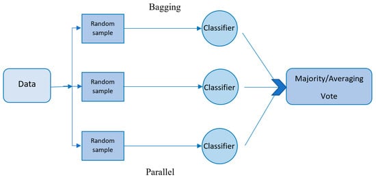
As depicted in Figure 1, in the bagging technique, the training data are partitioned into multiple subset sets, and the model is trained on each subset. The final prediction is then obtained by combining all individual outputs through majority voting (in classification problems) or average voting (in regression problems) ^{[21][34][35][36]}[21,34,35,36].

Figure 1. Visualization of the bagging approach.

Random Forest

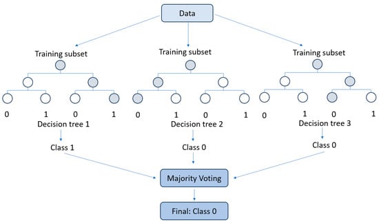
The concept of Random Forest was first introduced by Ho in 1995 [18] and has been the subject of ongoing improvements by various researchers. One notable advancement in this field was made by Leo Breiman in 2001 [19]. Random Forests are an ensemble learning technique for classification tasks that employs a large number of Decision Trees in the training model. The output of Random Forests is a class that is selected by the majority of the trees, as shown in Figure 2. In general, Random Forests exhibit superior performance compared to Decision Trees. However, the performance can be influenced by the characteristics of the data.

Figure 2. Visualization of the Random Forest classifier.

Random Forests utilize the bagging technique for their training algorithm. In greater detail, the Random Forests operate as follows: for a training set

{T S}_{n} = {(x_{1} . y_{1}) . \dots . (x_{n} . y_{n})}

, bagging is repeated B times, and each iteration selects a random sample with a replacement from

{T S}_{n}

and fits trees to the samples:

Sample $n$ $n$ training examples, $X_{b} . Y_{b}$ .
Train a classification tree (in the case of churn problems) $f_{b}$ $f_{b}$ on the samples $X_{b} . Y_{b}$ .

After the training phase, Random Forests can predict unseen samples

x^{'}

x^{'}

by taking the majority vote from all the individual classification trees

x^{'}

f^= 1 B \sum b = 1 B f b (x')

2.5.2. Boosting

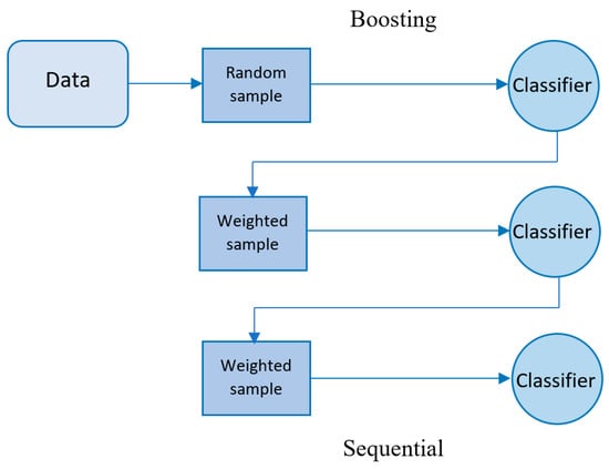
Boosting is another method for combining multiple base learners to construct a stronger model with more accurate predictions. The key distinction between bagging and boosting is that bagging uses a parallel approach to combine weak learners, while boosting methods utilize a sequential approach to combine weak learners and derive the final prediction, as shown in Figure 3. Like the bagging technique, boosting improves the performance of machine learning predictors, and in addition, it reduces the bias of the model [21].

Figure 3. Visualization of the boosting approach.

The Famous Trio: XGBoost, LightGBM, and CatBoost

Recently, researchers have presented three effective gradient-based approaches using Decision Trees: CatBoost, LightGBM, and XGBoost. These new approaches have demonstrated successful applications in academia, industry, and competitive machine learning [37]. Utilizing gradient boosting techniques, solutions can be constructed in a stagewise manner, and the over-fitting problem can be addressed through the optimization of loss functions. For example, given a loss function

ψ (y, f (x))

ψ (y, f (x))

and a custom base-learner h(x, θ) (e.g., Decision Tree), the direct estimation of parameters can be challenging. Thus, an iterative model is proposed, which is updated at each iteration with the selection of a new base-learner function h(x, θt), where the increment is directed by the following:

g t (x () = E y [\partial ψ (y, f (x (() \partial f (x () | x] f (x () = f ~ t - 1 (x)))))))

Hence, the hard optimization problem is substituted with the typical least-squares optimization problem:

(p t, θ t () = a r g m i n p, θ \sum_{i = 1 N [- g t (x i () + p h (x i, θ)] 2)})

Friedman’s gradient boost algorithm is summarized by Algorithm 1.

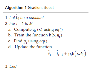
Algorithm 1 Gradient Boost

1: Let

{\hat{f}}_{0}

be a constant

2: For i = 1 to M

a . C o m p u t e g_{i} (x) u s i n g e q ()

b . T r a i n t h e f u n c t i o n h (x, θ_{i})

c . F i n d p_{i} u s i n g e q ()

d . U p d a t e t h e f u n c t i o n

{\hat{f}}_{i} = {\hat{f}}_{i - 1} + p_{i} h (x, θ_{i})

3: End

After initiating the algorithm with a single leaf, the learning rate is optimized for each record and each node ^[38][39][40][38,39,40]. The XGBoost method is a highly flexible, versatile, and scalable tool that has been developed to effectively utilize resources and overcome the limitations of previous gradient boosting methods. The primary distinction between other gradient boosting methods and XGBoost is that XGBoost utilizes a new regularization approach for controlling overfitting, making it more robust and efficient when the model is fine-tuned. To regularize this approach, a new term is added to the loss function as follows:

L (f () = \sum_{i = 1 n L (y^i, y i () + \sum_{m = 1 M Ω (δ m)})})

with

Ω (δ () = α |δ || + 0.5 β | |w || | 2||)

where w represents the value of each leaf, Ω indicates the regularization function, and |δ| denotes the number of branches. A new gain function is used by XGBoost, as follows:

G j = \sum_{i \in I j g i}

H j = \sum_{i \in I j h i}

G a i n = 1 2 [G L 2 H L + β + G R 2 H R + β - (G R + G)]

where

g i = \partial y^i L (y^i + y i)

and

h i = \partial y^i 2 L (y^i + y i)

The Gain represents the score of the no new child case, H indicates the score of the left child, and G denotes the score of the right child [41] .

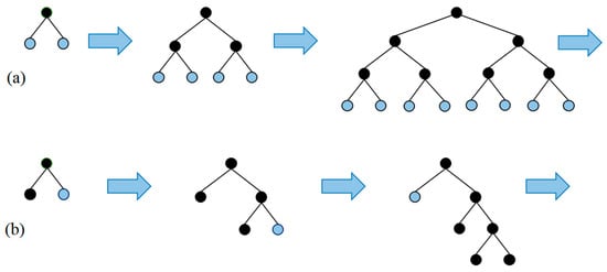
To decrease the implementation time, the LightGBM method was developed by a team from Microsoft in April 2017 [42]. The primary difference is that LightGBM Decision Trees are constructed in a leaf-wise manner, rather than evaluating all previous leaves for each new leaf (Figure 4a,b). The attributes are grouped and sorted into bins, known as the histogram implementation. LightGBM offers several benefits, including a faster training speed, higher accuracy, and the ability to handle large scale data and support GPU learning.

Figure 4. Comparison of tree growth methods. (a) XGBoost Level-wise tree growth. (b) LightGBM Leaf-wise tree growth.

The focus of CatBoost is on categorical columns through the use of permutation methods, target-based statistics, and one_hot_max_size (OHMS). By using a greedy technique at each new split of the current tree, CatBoost has the capability to address the exponential growth of feature combinations. The steps described below are employed by CatBoost for each feature with more categories than the OHMS (an input parameter):

To randomly divide the records into subsets,
To convert the labels to integer numbers,
To transform the categorical features to numerical features, as follows:

a v g T a r g e t = c o u n t I n C l a s s + p r i o r t o t a l C o u n t + 1

a v g T a r g e t = c o u n t I n C l a s s + p r i o r t o t a l C o u n t + 1

where totalCount denotes the number of previous objects, countInClass represents the number of ones in the target for a specific categorical feature, and the starting parameters specify prior ^[43].[43]