Your browser does not fully support modern features. Please upgrade for a smoother experience.
Please note this is a comparison between Version 1 by Anton Kovantsev and Version 2 by Fanny Huang.
The task of forecasting is a crucial topic with wide-range applications and significance in various fields. In fact, forecasting provides valuable insights into the future, helping individuals, organizations, and societies plan and adapt in a dynamic and uncertain world. Time series [1,2] and network link [3,4] are among the most significant and extensively investigated objects that have been the focus of forecasting efforts.
- predictability measures
- intrinsic predictability
- realized predictability
1. Introduction
Nowadays, the task of forecasting is a crucial topic with wide-range applications and significance in various fields. In fact, forecasting provides valuable insights into the future, helping individuals, organizations, and societies plan and adapt in a dynamic and uncertain world. Time series [1][2][1,2] and network link [3][4][3,4] are among the most significant and extensively investigated objects that have been the focus of forecasting efforts. The range of developed forecasting models is wide, starting from regression models [5] to neural networks [6] for time series forecasting, and from well-established classification methods [7] to random walks [8] for network links prediction.
Despite the extensive range of developed forecasting methods, researchers rarely address questions concerning the overall predictability of an object and its upper bound. Nevertheless, there are studies that delve into this matter, and the predictability measures they propose encompass a wide range, reflecting diverse viewpoints from various scientific domains, including dynamical systems [9] and information theory [10].
The concept of predictability is usually regarded from two sides [11]: with respect to a chosen forecasting model (realized predictability) and as a data property not depending on a certain model (intrinsic predictability).
2. Overview of Predictability Measures
The task of predicting the future has become a fundamental practice for many scientists across various disciplines. As a result, a multitude of forecasting methods have been devised, catering to a diverse array of objects and phenomena. This extensive range of objects has led researchers to explore predictive techniques in fields as varied as economics, climate science, medicine, social sciences, and more.
Among the various entities whose behaviors have been subject to prediction, time series [1][2][1,2] and network links [3][4][3,4] stand out as some of the most prominent and extensively studied. Time series, which represent a sequence of data points indexed by time intervals, find applications in fields such as finance [12][13], meteorology [13][14], and stock market analysis [14][15], where forecasting future values based on past observations is of paramount importance. Network links, on the other hand, are crucial in understanding and modeling the relationships and interactions among entities in complex systems, such as social networks [15][16], transportation networks [16][17], and biological systems [17][18].
Researchers can highlight certain methods that are widely utilized across diverse fields. Among these, linear and nonlinear regression models stand out as some of the most straightforward techniques. What makes them particularly appealing is their simplicity, as they do not demand significant computational resources and can be constructed without reliance on specialized tools or software. Regression models continue to find applications in research and practice, as evidenced by studies such as [5][18][19][5,19,20].
The autoregressive model ranks among the most popular forecasting methodologies, largely due to its well-defined algorithmic framework for model construction and parameter selection [20][21]. The research has seen extensive adoption of various autoregressive models, such as ARMA, ARIMA, ARCH, GARCH, and others, to predict a wide range of phenomena, such as market prices [14][21][22][23][15,22,23,24], network traffic [24][25][26][25,26,27], and social processes [27][28][29][28,29,30]. Oftentimes, hybrid autoregressive models that combine multiple forecasting techniques are used [30][31][32][33][31,32,33,34]. By combining the strengths of different methodologies, these hybrid approaches seek to harness the complementary predictive capabilities of various models, yielding more accurate and robust forecasts.
Neural networks represent a specific type of nonlinear functional architecture that involves iteratively processing linear combinations of inputs through nonlinear functions [34][35]. Artificial neural networks have found extensive application in various domains, demonstrating their efficacy in predicting stock prices and indices [6][35][36][6,36,37], addressing industrial challenges [37][38][39][38,39,40], facilitating medical forecasts [40][41][42][43][44][41,42,43,44,45], enhancing weather forecasts [45][46][47][48][46,47,48,49], and tackling a myriad of other challenges [49][50][51][50,51,52].
Well-established classification methods, including decision trees, k-Nearest Neighbors (k-NN), and Support Vector Machines (SVM), among others, have demonstrated their applicability in predicting links within a network [7], achieving competitive levels of accuracy. The utilization of these methods in link prediction tasks allows researchers to harness their robustness and adaptability to different datasets and graph structures. In the work of [52][53], a comparative analysis is conducted on various node similarity measures, encompassing both node-dependent indices and path-dependent indices. These measures serve as essential components in link prediction, aiding in quantifying the potential connections between nodes and guiding the predictive modeling process. Beyond these widespread techniques, there exist link prediction methods that leverage concepts such as random walks [8][53][8,54], matrix factorization [54][55][55,56], and others [56][57][58][57,58,59]. These methods are based on diverse mathematical frameworks to capture complex patterns within the network’s topology and provide valuable insights into the potential links between nodes.
The approaches discussed in the referenced papers are oriented towards the development of methods capable of making predictions with the desired level of quality on test datasets. However, it has been observed that authors often overlook certain questions: What is the overall predictability of this object? Can a model be devised that exhibits superior performance on this dataset?
To validate this concept, researchers introduce a citation network comprised of the regarded papers focused on forecasting and predictability assessment methods for various objects, such as time series and network links. The network and its connections are depicted in Figure 1. Notably, the figure illustrates that research studies aimed at enhancing forecast accuracy are rarely linked to predictability studies.
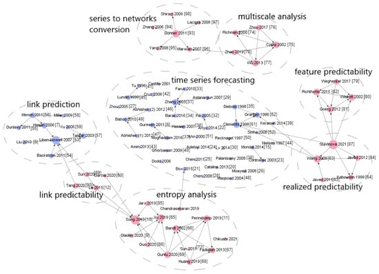
Figure 1. The citation network consisting of papers dedicated to forecasting and predictability assessment methods for different objects (time series, network links).
2.1. General Predictability Concepts
To evaluate the quality of predictive models on data, methods of predictability analysis for the modeling object can be employed. According to [11], the concept of object predictability should be divided into two components: realized predictability (RPr) and intrinsic predictability (IPr). The first type of predictability, realized predictability, is a function that depends on the forecasting model employed:
where m is the forecasting model and S is the object or class of objects. For example, different forecast quality metrics, such as MSE, MASE, RMSE, etc., are nothing but realized predictability measures. The second type, intrinsic predictability, is independent of the model used:
where S is the object or class of objects. Calculating theoretical estimates of intrinsic predictability for objects can be challenging, even in the case of simple data classes [59][60]. Therefore, the upper bound of realized predictability, which represents the predictability achieved by an optimal model, is used to estimate intrinsic predictability:
Low values of realized predictability could indicate not only the inherent complexity of the modeled object but also potentially inadequate quality of the selected model. Conversely, intrinsic predictability is independent of the forecasting model and can, therefore, be utilized to assess the data quality.
One of the central questions that motivated the experimental aspect of this study is how to establish a connection between quality measures (RPr), 𝜌𝑅, and a measure of intrinsic predictability, 𝜌𝐼. While researchers possess distinct tools for predictability estimation, the fundamental question is: do they truly have a meaningful relationship with each other?
Researchers have developed various approaches to measure the predictability of diverse objects, including univariate and multivariate time series, categorical time series (event sequences), network links, and more. It is important to note that there is not a singular methodological approach in this field, as different researchers approach this issue from the perspectives of various scientific domains, such as information theory, dynamical system theory, approximation theory, and others.
2.2. Time Series Predictability
Prior to discussing time series predictability measures, the notion of intrinsic unpredictability (IPr) concerning a random variable is focused on. The definition of an unpredictable random variable was introduced in reference [60][61]. A random variable 𝜉𝑡 is deemed unpredictable with respect to an information set Ω𝑡−1 if the conditional distribution 𝐹𝜉𝑡(𝜉𝑡|Ω𝑡−1) aligns with the unconditional distribution 𝐹𝜉𝑡(𝜉𝑡) of 𝜉𝑡, that is:
Specifically, when Ω𝑡−1 comprises past realizations of 𝜉𝑡, Equation (4) suggests that having knowledge about these past realizations does not enhance the predictive accuracy of 𝜉𝑡. It is important to note that this form of unpredictability in 𝜉𝑡 is an inherent attribute, unrelated to any prediction algorithm.
2.2.1. Univariate Time Series
Methods for estimating univariate time series predictability can be categorized into two groups: methods for estimating sample predictability and methods for estimating intrinsic predictability. The first group of methods aims to evaluate realized predictability (RPr) and encompasses measures that analyze forecast quality. The second group comprises intrinsic predictability (IPr) estimation methods, which are often rooted in information theory approaches, particularly those involving Shannon entropy.
The starting point for developing sample predictability measures is the work of [61][62], in which the predictability of a time series generated by a wide-sense stationary process is proposed to be evaluated as the ratio of the theoretical optimal forecast and the original time series variances. Consequently, computing predictability values requires knowledge of the optimal forecast, which is challenging to obtain for real-world time series. Therefore, coefficients for the sample predictability estimation (RPr), based on the approach from [61][62], are developed [62][63]. The approach from [61][62] assesses predictability as the ratio of the optimal forecast and the original series variances, but instead of using the optimal forecast error, while the proposed approach from [62][63] employs the forecast error shown by a specific model. Thus, the coefficient of efficiency (CE) indicates the ratio of the sample variance of the model’s forecast error to the sample variance of the time series, measured over the entire observation period. The seasonally adjusted coefficient of efficiency (SACE) differs from CE in that the series variance is considered within a specific season. The SACE coefficient is useful for time series where the mean value changes based on the season.
Furthermore, this group includes the work [63][64], which introduces a metric of realized predictability based on the ratio of two values: the sum of squared errors in the case of forecasting the original time series and the case of forecasting the same series after random shuffling. It is evident that measuring the predictability of a series using the three mentioned measures is entirely dependent on the model’s performance, and therefore, does not provide insight into the intrinsic predictability of the data.
The second group of methods for analyzing the predictability of univariate time series is based on (but not limited to) estimating various forms of entropy for the series, thereby allowing the assessment of data properties rather than models. This group of methods, in turn, is further divided into two subgroups: methods for assessing the predictability of the entire series and methods for assessing predictability on specific scales. Different scales of the series refer to series obtained from the original by retaining only those values that occur at specific intervals of time. Investigating the predictability of the series at different scales can provide valuable information about long-term correlations in the data, which can subsequently be utilized in training predictive models.
2.2.2. Multivariate Time Series
The goal of assessing the predictability of components within a multivariate time series (also referred to as features) is to select a set of features that best describe the behavior of the object and enable the model to make forecasts of the desired quality. In fact, there may be situations where using a particular feature as a predictor does not improve the forecast quality, complicating the search for patterns in the data. When dealing with large volumes of input data, there arises a need to match the original features with a specific subset of smaller-sized features that can make the model’s forecasts more stable and effective. However, standard dimensionality reduction methods are focused on preserving data properties unrelated to predictability, which introduces the risk of losing important information contained within the data [64][79].
There is an entire group of methods [64][65][66][67][79,80,81,82] in the field of extracting predictable features from multivariate time series. All works within this group share a similar algorithm. The input consists of multivariate time series, and the objective is to find a mapping from a space whose dimension equals the number of series components to a lower-dimensional space. The principle of dimensionality reduction may vary depending on the algorithm, yet all methods boil down to an optimization problem. The approach [67][82] is aimed at theoretically assessing realized predictability, while the other works within this group deal with the intrinsic predictability of features.
Indeed, in [65][80], a method for extracting slowly changing (or invariant) features, known as Slow Feature Analysis (SFA), is proposed. This method is utilized to analyze multivariate time series containing sensor data. The principle of feature extraction for creating a lower-dimensional space involves retaining those features that change over time as slowly as possible. Ultimately, the dimensionality reduction task is reduced to a variational calculus optimization problem.
The Forecastable Component Analysis (ForeCA) method [66][81] also addresses the task of feature selection, in this case, forecastable features. The work introduces a measure of predictability for time series generated by stationary random processes. The calculation of this measure employs the entropy of the process, which, in turn, is determined using spectral density. The ultimate task of finding features is reduced to maximizing this predictability measure.
A similar task of finding a set of features is considered in [67][82] (Predictable Feature Analysis, PFA), with the distinction that feature selection is carried out considering a specific model (i.e., the features that are well predicted by it). A criterion is derived that the model must adhere to in order to be used with PFA. It is worth noting that despite analyzing a specific model, this method examines theoretical predictability without utilizing forecast results. The advantage of this approach is the knowledge of a certain model that is able to make the predictions of the desired quality. However, the optimization problem is more challenging than in SFA: the forecasting optimization problem is embedded within the optimization problem of searching for predictable features.
The method from [64][79] (Graph-based Predictable Feature Analysis, GPFA) is based on interpreting predictability as a situation where the variance of a time series in the next time step is small given that the current value of the series is known. The dimensionality reduction task is formulated as the search for an orthogonal transformation of the original series. The term graph in the method’s name is mentioned simply because it is used as an auxiliary tool to search for the columns of the orthogonal transformation matrix. Additionally, the predictable components of a multivariate series can be seen as neighboring nodes on a specific graph, connected by an edge.
All the methods discussed (apart from [67][82] that theoretically assesses realized predictability) are aimed at estimating intrinsic feature predictability. Additionally, there exists a straightforward approach to estimate realized feature predictability [68][69][83,84]. This approach identifies the most useful features for predicting the remaining time of system performance. The predictability measure is defined as a function dependent on the prediction horizon, model class, model parameters, and the required accuracy threshold. The proposed predictability measure combines the threshold and the accuracy achieved by the model into a single value ranging from 0 to 1. Subsequently, pairs (a set of features and a model) with a favorable predictability value are selected through brute force.
2.2.3. Categorical Time Series
In practice, these time series can be referred to as events or event sequences. For instance, in [70][85], sequences composed of items viewed or purchased by users during a single session on a retailer’s website are considered. Predictability in this context refers to the probability of correctly determining the next element in the sequence (i.e., the purchase of a specific item), given the session’s start and the user’s session history. The authors provide an estimation of the maximum theoretical predictability of the sequence, expressed using entropy as formulated in [10]. Furthermore, the theoretical predictability realized by specific algorithms (RPr) is assessed by analyzing potential algorithm outcomes and selecting the result with the best forecasting quality. For instance, in the case of a Markov chain model, predictability is evaluated as the proportion of observations where the most likely transition from one state to another occurred. Thus, theoretical predictability can only be assessed for explicit models. Estimating the theoretical predictability for black-box models using this approach is not feasible.
In Reference [71][86], the authors consider the problem of forecasting the next point in a trajectory (the category of the point, not its coordinates). Similar to [71][86], the maximum theoretical predictability of the sequence is assessed using the entropy formula from [10]. Additionally, two statistics are introduced to measure the gap between theoretical predictability (IPr) and the maximum prediction accuracy achieved using a set of models (3).
In [72][73][87,88], the authors assess the realized predictability (RPr) of client’s transactional sequences by employing a coefficient based on the mean absolute error of the selected predictive model for each sequence. Subsequently, they categorize all sequences into predictability classes based on the values of the predictability measure. This approach can be utilized to gauge the predictability level of a sequence prior to forecasting, by utilizing a form of meta-classifier that assigns categorical time series to their corresponding predictability classes. Experiments demonstrated the efficiency of this approach, as the estimated predictability classes consistently align with those obtained through the application of a prediction model. The further development of this concept is done in [Koshkareva, 2023], which shows that customer separation by predictability levels helps to improve the forecasting quality of the whole population due to the decomposition of all clients’ time series, and that forecasting failures caused by environmental instability, like pandemics or military action, can be leveled out by means of this approach.
2.3. Network Link Predictability
Most of the studies on network link predictability discussed are focused on assessing intrinsic predictability. In Reference [74][12], a network is considered predictable if the removal or addition of a small number of randomly chosen nodes preserves its fundamental structural characteristics. Such networks are referred to as structurally consistent. The proposed measure is the Universal Structural Consistency Index, which is based on perturbing the adjacency matrix and evaluates the corresponding changes in network structural features. Through conducted experiments, a strong correlation is revealed between link prediction accuracy and the structural consistency index in various real-world networks, demonstrating the applicability of network structural consistency as a link predictability assessment. Moreover, this index can be used in tasks of missing links prediction. Such experiments with networks constructed using the Erdos–Renyi model indicate, as expected from the networks’ construction, that this type of networks is poorly predictable.
Furthermore, to assess the predictability of network structure, the normalized shortest compression length of the network structure can be employed [75][89]. Any network can be transformed into a binary string through compression. The length of the string increases as the randomness in the network structure grows. The authors compared their proposed predictability measure with the accuracy of the best available link prediction algorithm (as an approximation of the optimal algorithm) estimated via performance entropy and find a strong correlation.
Another work focusing on the assessment of the intrinsic predictability of network links is [59][60]. By considering ensembles of well-known network models, the authors analytically demonstrated that even the best possible link prediction methods provide limited accuracy, quantitatively dependent on the ensemble’s topological properties such as degree heterogeneity, clustering, and community structure. This fact implies an inherent limitation on predicting missing links in real-world networks due to uncertainty arising from the random nature of link formation processes. The authors show that the predictability limit can be estimated in real-world networks and propose a method to approximate this limit for real-world networks with missing links. The predictability limit serves as a benchmark for evaluating the quality of link prediction methods in real-world networks. Additionally, the authors conducted experiments comparing their proposed predictability measure with the structural consistency index from [74][12].
The authors of [76][90] assessed the predictability of links in temporal networks. The temporal nature of links in many real-world networks is not random, but predicting them is complicated due to the intertwining of topological and temporal link patterns. The paper introduces an approach based on Entropy rate, which combines both topological and temporal patterns to quantitatively assess the predictability of any temporal network (in previous works, only temporal aspects were considered). To examine both topological and temporal properties of the network, the sequence of adjacency matrices is treated as realizations of a random process. The subsequent procedure is similar to the one in [10] for trajectory predictability estimation: the entropy rate and theoretical upper bound of intrinsic predictability are derived, and then applying the Lempel–Ziv–Welch data compression algorithm yields an expression for the approximate entropy value. It is noted that for most real-world temporal networks, despite the increased complexity of predictability estimation, the upper bound of combined topological-temporal predictability is higher than that of temporal predictability.
Furthermore, there are two studies [77][78][91,92] focusing on the realized predictability of network links; specifically, the predictability observed through a selected feature-based link prediction model. The authors evaluate link predictability by assessing the error of the chosen model and divide the links within a small portion of the network into high and low predictability classes based on the error value. Subsequently, they train a meta-classifier on this subset of the network to estimate the predictability class using certain link features. This meta-classifier can then be applied to the entire network to estimate link predictability without the time-consuming process of training a link prediction model.
Moreover, there are methods that involve converting time series into networks. These methods can be categorized into three classes based on the type of resulting network [79][93]: (a) proximity networks; (b) visibility networks; (c) transition networks. The first category of methods constructs networks by utilizing information about the mutual proximity of various segments within time series. Mutual proximity can be measured in various ways, such as through the correlation between time series cycles (resulting in a cycle network [80][94]), the correlation between time series segments (resulting in a correlation network [81][95]), or the closeness of time series segments in phase space (resulting in a recurrence network [82][96]). The second category, known as visibility network methods, generates networks based on the convexity of consecutive observations in series [83][97]. Lastly, the class of methods producing transition networks constructs networks by considering the transition probabilities between groups of aggregated values from series [84][98].
However, there is only one study [85][99] that analyzed predictability under such transformations. The authors utilized the transition network approach to convert time series into networks. They then calculated network characteristics and employ them for clustering time series into two groups. By measuring the forecasting errors obtained by various models on time series from these clusters, they concluded that these clusters can be considered as classes of high and low predictability, as the mean forecasting error in one class is significantly lower than in the other.
2.4. Overview Summary
To assess the predictability of data, there is a multitude of measures that allow working with various objects: univariate and multivariate time series, categorical time series (sequences of events), and network links. In the case of time series, measures are developed to evaluate the predictability of the series as a whole, as well as at specific scales. The diversity of measures presented in the studies is due to researchers expressing their perspectives on predictability assessment from various scientific domains, such as information theory, dynamical systems, approximation theory, and so on. However, despite the variety of existing predictability measures, the challenge of proper analysis of connection between intrinsic and realized predictability remains unresolved.