2. DNA Microarrays

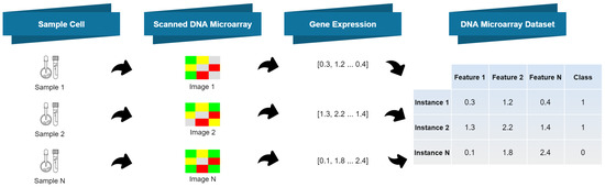
2.1. DNA Microarrays: Acquisition Technique and Resulting Data

• It is composed by a solid surface, arranged in columns and rows, containing thousands of spots;
• Each spot refers to one single gene and contains multiple strands of the same DNA, yielding a unique DNA sequence;
• Each spot location and its corresponding DNA sequence is recorded in a database.

Figure 1. Overview of the DNA microarray technique data acquisition from samples ^[2][4].

1.

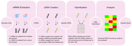
Extraction of ribonucleic acid (RNA) from the sample cells and drawing out the messenger RNA (mRNA) from the existing RNA, because only the mRNA develops gene expression.

2.

CDNA creation: a DNA copy is made from the mRNA using the reverse transcriptase enzyme, which generates the complementary DNA (CDNA). A label is added in the CDNA representing each cell sample (e.g., with fluorescent red and green for cancer and healthy cells, respectively). This step is necessary since DNA is more stable than RNA and this labeling allows identifying the genes.

3.

Hybridization: both CDNA types are added to the DNA microarray and each spot already has many unique CDNA. When mixed together, they will base-pair each other due to the DNA complementary base pairing property. Not all CDNA strands will bind to each other, since some may not hybridize being washed off.

4.

Analysis: the DNA microarray is analyzed with a scanner to find patterns of hybridization by detecting the fluorescent colors.

The following are possible outcomes of the analysis stage:

• A few red CDNA molecules bound to a spot, if the gene is expressed only in the cancer (red) cells;
• A few green CDNA molecules bound to another spot, if the gene is expressed only in the healthy (green) cells;
• Some of both red and green CDNA molecules bound to a single spot on the microarray, yielding a yellow spot; in this case, the gene is expressed both in the cancer and healthy cells;
• Finally, several spots of the microarray do not have a single red or green CDNA strand bound to them; this happens if the gene is not being expressed in either type of cell.

On the one hand, the red color flags the higher production of mRNA in the cancer cell as compared to the healthy cell. On the other hand, the green color states that people have a larger production of mRNA in the healthy cell, as compared to the cancer cell. However, a yellow spot suggests that the gene is expressed equally in both cells and therefore it is not related with the disease, because when the healthy cell becomes cancerous its activity does not change. Figure 2 depicts the process of generating a dataset using the DNA microarray technique summarized in Figure 1.

Figure 2. Dataset generation with gene expression data from DNA microarray data acquisition ^[2][4].

2.2. Feature Discretization

DNA microarray datasets are composed of high dimensionality numeric feature vectors. These features contain a large amount of information regarding gene expressions, but they also contain irrelevant fluctuations (noise) ^[3][10], which may be harmful for the performance of ML algorithms. The use of FD techniques, which convert continuous (numeric) features into discrete ones, may yield compact and adequate representations of the microarray data, with less noise ^[4][5][11,12]. In other words, FD aims at finding a representation of each feature that contains enough information for the learning task at hand, while ignoring minor fluctuations that may be irrelevant for the task at hand. FD methods can be supervised or unsupervised, depending on whether label information is used or not, respectively ^[4][11]. The Equal Frequency Binning (EFB) method ^[6][13], which is unsupervised, discretizes continuous features into a given number of intervals (bins), which contain approximately the same number of instances. The Unsupervised Linde-Buzo-Gray 1 (U-LBG1) method discretizes each feature into a specified number of intervals, by minimizing the Mean Squared Error (MSE) between the original and the discretized feature. The number of intervals may be decided by demanding that the MSE be lower than some threshold (Δ) or by specifying the maximum number of bits per feature (q). The supervised Minimum Description Length Principle (MDLP) method recursively divides the feature values into multiple intervals, using an information gain minimization heuristic (entropy). Please refer to ^[7][14] for a formal description of this method and to ^[6][8][5,13] for additional insights on other FD approaches.

2.3. Feature Selection

In the presence of high-dimensional data, dimensionality reduction techniques ^[9][10][9,15] are often essential to obtain adequate representations of the data and to improve the ML models results, effectively addressing the “curse of dimensionality”. One type of dimensionality reduction technique that has been successful with microarray data is FS ^[9][10][9,15]. FS techniques select a subset of features from the original set by following some selection criterion. One way to perform FS is to rank the features according to their relevance, assessed by a given function, which can also be supervised (if it uses label information) or not. For microarray data, the use of FS techniques is also known as Gene Selection (GS). Some well-known methods that have been used for microarray data are the following:

• Unsupervised methods—Laplacian Score (LS) ^[11][16], spectral (also known as SPEC) ^[12][17], and term-variance ^[13][18];
• Supervised methods—Fisher Ratio (FiR) ^[14][19], Fast Correlation-Based Filter (FCBF) ^[15][20], Maximum Relevance Minimum Redundancy (MRMR) ^[16][21], ReliefF ^[17][22], and Relevance-Redundancy Feature Selection (RRFS) ^[18][23].

The RRFS method can also work in unsupervised mode using the mean-median (MM) relevance metric, defined, for the i-th feature, as

$${\mathrm{MM}{i}_{}=|{\overline{X}}_i-\mathrm{median}(X_i\left)\right|,}_{}$$

with ${\overline{X}}_i$ denoting the mean of the i-th feature. In supervised mode, RRFS uses as relevance measure the Fisher ratio ^[14][19], also known as Fisher score, defined as (for the i-th feature) 

$${\mathrm{FiR}{i}_{}=\frac{\left|{\overline{X}}_i^{(-1)\frac{\left|{}_{}^{}-{\overline{X}}_i^{\left(1\right)\frac{\left|{}_{}^{}\right|}{\sqrt{\mathrm{var}{\left(X_i\right){(-1){}^{}+\mathrm{var}{\left(X_i\right){\left(1\right){}^{}\frac{\sqrt{}}{},}^{}}^{}}^{}}^{}}}}\right|}{}}\right|}{}}_{}$$

where ${\overline{X}}_i^{(-1)}$ , ${\overline{X}}_i^{\left(1\right)}$ , and $\mathrm{var}{\left(X_i\right){(-1){}^{}}^{}}^{}$ are the sample means and variances of feature $X_i$ , for the patterns of each of the two classes (denoted as −1 and 1). This ratio measures how well each feature alone separates the two classes ^[14][19], and has been found to serve well as a relevance criterion for FS tasks. For more than two classes, FiR for feature $X_i$ is generalized ^[19][20][6,24] as 

$${\mathrm{FiR}{i}_{}=\frac{{\displaystyle \sum _{j=1\underset{}{\overset{}{c}}{\mathrm{n}}_j{\left({\overline{X_i}}^{\left(j\right){\left({\left(-\overline{X_i}\right)}^2\right)}^{}\frac{{\displaystyle }}{{\displaystyle \sum _{j=1\underset{}{\overset{}{c}}{\mathrm{n}}_j\mathrm{var}\left(X_i^{\left(j\right)\left({}_{}^{}\right)\frac{{\displaystyle }}{},}\right)}^{}}}}\right)}^{}}^{}}}{}}_{}$$

where c is the number of classes, $n_j$ is the number of samples in class j, and ${\overline{X_i}}^{\left(j\right)}$ denotes the sample mean of $X_i$ considering only samples in class j; finally, $\overline{X_i}$ . Among many other applications, the Fisher ratio has been used successfully with microarray data, as reported by Furey et al. ^[21][25]. When using the Fisher ratio for FS, we simply keep the top-rank features.

2.4. Classifiers

2.4.1. SVM

SMVs ^{[22][23][24][25]}[33,34,35,36] follow a discriminative approach to learn a linear classifier. As is well-known, a non-linear SVM classifier can be obtained by the use of a kernel, via the so-called kernel trick ^[22][33]: since the SVM learning algorithm only uses inner products between feature vectors, these inner products can be replaced by kernel computations, which are equivalent to mapping those feature vectors into a high-dimensional (maybe non-linear) feature space. With a separable dataset, a SVM is learned by looking for the maximum-margin hyperplane (a linear model) that separates the instances according to their labels. In the non-separable case, this criterion is relaxed via the use of slack variables, which allow for the (penalized) violation of the margin constraint; for details, see ^[24][25][35,36]. SVMs are well suited for high-dimensional problems. Although the original SVM formulation is inherently two-class (binary), different techniques have been proposed to generalize SVM to the multi-class case, such as one-vs-rest (or “one-versus-all”) and one-vs-one ^[26][27][37,38].

2.4.2. DT

DT classifiers ^[22][33] also adopt a discriminative approach. A DT is a hierarchical model, in which each local region of the data is classified by a sequence of recursive splits, using a small number of partitions. The DT learning algorithm analyzes each (discrete or numeric) feature for all possible partitions and choose the one that maximizes one of the so-called impurity measures. The tree construction proceeds recursively and simultaneously for all branches that are not yet pure enough. The tree is complete when all the branches are considered pure enough, that is, when performing more splits does not improve the purity, or when the purity exceeds some threshold. There are several algorithms to learn a DT. The most popular are the Classification and Regression Trees (CART) ^[28][39], the ID3 algorithm ^[29][40] and its extension, the well-known C4.5 ^[30][31][41,42] algorithm. A survey of methods for constructing DT classifiers can be found in ^[32][43], which proposes a unified algorithmic framework for DT learning and describes different splitting criteria and tree pruning methods. DT are able to effectively handle high-dimensional and multi-class data.

2.5. Related Approaches

Many unsupervised and supervised FD and FS techniques have been employed on microarray data classification for cancer diagnosis ^[1][33][34][1,44,45]. Since microarray datasets are typically labeled, the use of supervised techniques is preferred, as supervised methods normally outperform unsupervised ones. Some unsupervised FD techniques perform well when combined with some classifiers. For instance, the Equal Frequency Binning (EFB) technique followed by a Naïve Bayes (NB) classifier produces very good results ^[35][46]. It has also been reported that applying Equal Interval Binning (EIB) and EFB with microarray data, followed by SVM classifiers, yields good results ^[36][47]. It has also been shown that FS significantly improves the classification accuracy of multi-class SVM classifiers and other classification algorithms ^[37][48]. An FS filter (i.e., a FS method that is agnostic to the choice of classifier that will be subsequently used) for microarray data, based on the information-theoretic criterion named Double Input Symmetrical Relevance (DISR) was proposed by ^[36][47]. The DISR criterion is found to be competitive with existing unsupervised FS filters. The work in ^[38][49] explores FS techniques, such as backward elimination of features, together with classification using Random Forest (RF) ^[39][50]. The authors concluded that RF has better performance than other classification methods, such as Diagonal Linear Discriminant Analysis (DLDA), K-Nearest Neighbors (KNN), and SVM. They also showed that their FS technique led to a smaller subset of features than alternative techniques, namely Nearest Shrunken Centroids (NSC) and a combination of filter and nearest neighbor classifier. The work in ^[40][51] introduced the use of Large-scale Linear Support Vector Machine (LLSVM) and Recursive Feature Elimination with Variable Step Size (RFEVSS), improving the Recursive Feature Elimination (SVMRFE) technique. The improvement upgrades RFE with a variable step size, to reduce the number of iterations (in the initial stages in which non-relevant features are discarded, the step size is larger). The standard SVM is upgraded to a large-scale linear SVM, thus accelerating the method of assigning weights. The authors assess their approach to FS with SVM, RF, NB, KNN, and Logistic Regression (LR) classifiers. They conclude that their approach achieves comparable levels of accuracy, showing that SVM and LR outperform the other classifiers. Recently, in the context of cancer explainability, the work in ^[41][52] considered the problem of finding a small subset of features to distinguish among six classes. The goal was to devise a set of rules based on the most relevant features that can distinguish classes based on their gene expressions. The proposed method combines a FS-based Genetic Algorithm (GA) with a fuzzy rule-based system to perform classification on a dataset with 21 instances, more than 45,000 features, and six classes. The proposed method generates ten rules, with each one addressing some specific features, making them crucial in explaining the classification results of ovarian cancer detection. A survey of common classification techniques and related methods to increase their accuracy for microarray analysis can be found in ^[1][33][1,44]. The experimental evaluation is carried out in publicly available datasets. The work in ^[42][53] surveys the use of FS techniques for microarray data. For other related surveys, please see ^{[40][43][44][45]}[51,54,55,56].