Your browser does not fully support modern features. Please upgrade for a smoother experience.
Please note this is a comparison between Version 1 by Xichuan Liu and Version 2 by Sirius Huang.
As rainfall exhibits high spatiotemporal variability, accurate and real-time rainfall monitoring is vitally important in fields such as hydrometeorological research, agriculture and disaster prevention and control. The utilization of commercial microwave links (CMLs) for rainfall estimation, as an opportunistic sensing method, has generated considerable attention. Relying on CML networks deployed and maintained by mobile network operators can provide near-surface precipitation information over large areas at a low cost.
- commercial microwave links (CMLs)
- opportunistic sensing
- rainfall estimation
- environment monitoring
- remote sensing
1. Background
Precipitation, as one of the most significant links in the Earth’s water cycle, is intimately associated with people’s lives. The spatial and temporal heterogeneity of precipitation development is the main cause of natural disasters such as droughts, floods and mudslides [1]. Accurate monitoring of precipitation has significant implications in fields such as agriculture, hydrometeorological research and water resource management.
Currently, meteorological operations mainly rely on rain gauges, weather radar and meteorological satellites to measure precipitation. However, due to the inherent limitations of these dedicated rain sensors, quantitative precipitation products still cannot satisfy the requirements of comprehensive meteorological observations, especially as global warming may lead to more extreme precipitation events [2]. Rain gauges, which are believed to provide point measurements of surface rainfall, are unsuitable for constructing a monitoring network due to their low spatial representativeness. In addition, wind and splash effects introduce uncertainties in its measurement [3]. Contrary to rain gauges, based on the statistical power–law relationship between the radar reflectivity Z and the rain rate R, weather radar allows for quantitative precipitation estimation (QPE) over large areas. However, the parameters of the Z–R relationship are highly sensitive to the raindrop size distribution (DSD) associated with precipitation types, geographical locations and climatic characteristics, which may cause large systematic biases [4]. Other uncertainty sources include ground clutter, beam blockage, bright bands and the vertical variability of the precipitation system [5]. As meteorological satellite technology matures, satellites can measure precipitation almost globally, which is especially important in areas where radar and rain gauges are not available [6]. However, subject to low spatial and temporal resolution, satellite products are not available for small-scale hydrological applications, such as catchment modeling in urban and mountainous areas. Moreover, although several satellite-based rainfall inversion algorithms have been developed [7][8][7,8], the accuracy of their estimates still needs to be improved [9].
Consequently, the concept of opportunistic rainfall measurement methods emerged, and the potential of devices such as commercial microwave links (CMLs) [10], personal weather stations [11], vehicle windscreen wipers [12] and street cameras [13] has been successively explored. These methods can provide additional precipitation information and promise to improve dedicated precipitation products, with CMLs being one that has the most prospective application. Based on existing CML networks built and maintained by mobile network operators, it can provide alternative precipitation observations in a cost-effective manner in areas lacking rain sensors [14] or additional precipitation information in areas with existing rainfall observations to enhance the spatial and temporal resolution as well as the accuracy of precipitation products [15][16][15,16].
2. Procedures in Deriving Rainfall Maps from Attenuation
When the path of CMLs is exposed to rainfall, additional attenuation of the microwave signal occurs accordingly. However, these attenuation increments are not entirely due to scattering and absorption by raindrop particles. Phenomena such as electronic component drift, changes in water vapor, multipath effects, and wet antenna effects can also lead to changes in signal quality. Deriving rainfall estimates from CML attenuation is, therefore, a sophisticated process, which is described in detail in this section.2.1. Classification of Dry and Wet Periods
As mentioned above, phenomena other than or triggered by rainfall may also cause signal impairment. Therefore, when we obtain attenuation data for CMLs, typically the transmitted signal level (TSL) minus the received signal level (RSL), the first critical issue is to determine at each timestamp whether the CMLs are affected by rainfall. More simply, the CML data need to be classified into dry (rain free) and wet (rainy) periods. In order to accomplish the classification of dry and wet periods, scholars have developed a variety of methods, which can be broadly divided into three categories. The first category is based on the analysis of attenuation sequences to determine whether rainfall exists on the path of CMLs. The simplest way to distinguish between dry and wet periods is based on a global threshold for attenuation, with periods above the threshold being treated as wet [17][44]. Rahimi et al. [18][23] found that RSL sequences of dual-frequency microwave links are highly correlated during wet periods and suggested setting correlation thresholds to distinguish between dry and wet periods. Further, Overeem et al. [19][45] extended the spatial correlation of rainfall from individual CMLs to all CMLs within a certain range and proposed the so-called nearby link approach (NLA). They considered a time period as wet if the RSLs of at least half of the CMLs in the range decreased simultaneously during that time period. In addition, Schleiss et al. [20][27] found significant differences in the local variability of signal attenuation between dry and wet periods and proposed the use of a rolling window to calculate the standard deviation of the attenuation sequence to identify dry and wet periods based on a predetermined threshold. Recently, Graf et al. [21][46] proposed an improved version of this algorithm, arguing that the threshold can depend on the fluctuating trend of individual CMLs rather than only on climatology. Based on the short-time Fourier transform of the RSL sequence, Chwala et al. [22][28] found that the normalized amplitude difference between low and high frequencies of the power spectrum can be used to determine the dry and wet periods. The second category of classification methods relies on dedicated rainfall observations in the vicinity of CMLs. As near-surface rainfall measurement instruments, rain gauges are widely used to achieve dry/wet period classification for CMLs [23][24][47,48]. In the literature [25][49], considering the elevation angle of the radar, if the path-averaged rain rate of the radar QPE is greater than 0.1 mm/h, the current and subsequent time steps are regarded as wet periods. Kumah et al. [26][27][50,51] utilized Meteosat Second Generation satellites to check for the presence of rain areas in the path of CMLs. The last category is data-driven approaches based on machine learning. Thanks to the massive data, they can derive hidden feature information to explore patterns of signal fluctuations and apply them to dry and wet period classification. Reller et al. [28][52] demonstrated the applicability of a factor graph-based quasi-periodic signal model for dry and wet period classification. The literature [29][30][53,54] reported cases where Markov models were employed to determine dry and wet periods. In addition, dry/wet classification based on the multifamily likelihood ratio test [31][55] and the kernel Fisher discriminant analysis [32][56] have been attempted. Subsequently, time-delay neural networks [33][57], long short-term memory neural networks (LSTM) [34][35][58,59], support vector machines (SVM) [36][60] and convolutional neural networks (CNN) [37][61] are also used for dry and wet period identification for CMLs. In [38][62], the dry and wet period classification performance of several machine learning models was compared and the ensemble machine learning classifier was recommended as the preferred one. Additional information on existing dry and wet period classification algorithms can be found in Table 1.Table 1.
Existing techniques for dry and wet period classification.
| Authors and Year | Country | Highlights |
|---|---|---|
| Rahimi et al. (2003) [18][23] | England | The RSL sequences of dual-frequency CMLs were found to increase in correlation during the wet period, and a correlation threshold was used to distinguish between dry and wet periods. The classification method detected approximately 80% of dry periods and 92.5% of wet periods. |
| Upton et al. (2005) [24][48] | England | Rain gauge data in the vicinity of CMLs were used to differentiate between dry and wet periods and compared with the classification method of dual-frequency CMLs. The use of nearby rain gauge data could well improve the dry and wet period classification of dual-frequency CMLs. |
| Leijnse et al. (2007) [17][44] | The Netherlands | Based on the historical data, a simple global threshold was constructed and the portion above the threshold was treated as wet periods. |
| Schleiss et al. (2010) [20][27] | France | Based on the different local variability of dry/wet period attenuation, the standard deviation of attenuation was calculated using a rolling window to differentiate between dry and wet periods according to a preset threshold. On average, 92% of wet periods, 86% of dry periods and 93% of total rainfall were identified. |
| Overeem et al. (2011) [25][49] | The Netherlands | Radar data were used to distinguish between dry and wet periods; considering that the correlation of RSL sequences of nearby CMLs in wet periods rises, the nearby link approach (NLA) was proposed to distinguish between dry and wet periods. Both radar and NLA were able to invert rainfall accurately with similar results. |
| Reller et al. (2011) [28][52] | Switzerland | The Gaussian factor graph was used to distinguish between the dry and wet periods. Case studies showed that the proposed method has a high classification performance. |
| Chwala et al. (2012) [22][28] | Germany | Due to the significant increase in the high-frequency components of the signal during the wet period, a spectral analysis method based on the short-time Fourier transform was proposed to classify dry and wet periods. The weighted mean error rate of the classification results was as low as 0.098. |
| Wang et al. (2012) [30][54] | Switzerland | A Markov switching model was used to differentiate between dry and wet periods, which was compared with rolling standard deviation, factor graphs and the global threshold method. The false-positive and false-negative rates were about 8% and 15%, respectively, in the case of a stationary baseline. In the case of an unstable baseline, the false-positive and false-negative rates were about 5% and 23%, respectively. |
| Rayitsfeld et al. (2012) [29][53] | Israel | A Hidden Markov Model was used to determine the dry and wet periods. Rainfall inversions using this method showed good correlation and low bias compared with rain gauge results. |
| Cherkassky et al. (2012) [39][63] | Israel | Based on the statistical characteristics of attenuation, a linear Fisher’s discriminant was used to distinguish between dry and wet periods and was able to identify 83% of wet periods, with a false-positive rate of 12%. |
| Harel et al. (2013) [31][55] | Israel | An algorithm based on a multifamily likelihood ratio test was used to separate dry and wet periods, and the true-positive rate could reach about 90%. |
| Dordević et al. (2013) [33][57] | Germany | Focused time-delay neural networks were used to distinguish between dry and wet periods. The average test error of the classification results was only 1.1095%, with a correlation coefficient of 0.9647. |
| Cherkassky et al. (2014) [32][56] | Israel | Based on the statistical characteristics of attenuation, the kernel Fisher’s discrimination was used to distinguish dry and wet periods. The results showed that the classification accuracy could reach 85.35%. |
| He et al. (2019) [35][59] | China | A dry and wet period classification algorithm based on LSTM was proposed. The daily classification accuracy exceeded 60%, with some results achieving up to 98%. |
| Polz et al. (2020) [37][61] | Germany | A dry and wet period classification algorithm based on CNN was proposed. An average of 76% wet periods and 97% dry periods were detected in the validation results. |
| Song et al. (2020) [36][60] | China | SVM was used to distinguish between dry and wet periods based on statistical features of attenuation. The classification accuracy exceeded 0.8 and the majority of the outcomes displayed true-positive and false-positive rates that exceeded 0.9 and were less than 0.2, respectively. |
| Kumah et al. (2020) [26][50] | Kenya | Satellite data were used to identify rain areas along the CML path. The accuracy of rainfall inversion for CMLs supported by satellite data was high. |
2.2. Determination of Baseline
After the classification of dry and wet periods, the wet period attenuation cannot be used directly for rainfall inversion; instead, the baseline attenuation (also known as the zero-level attenuation), which consists mainly of free-space losses and gas attenuation, needs to be removed from the wet period attenuation. Considering the generally short duration of rainfall, a common assumption is that factors affecting baseline attenuation may differ little between the wet period and the preceding dry period. Thus, the baseline can be set as the most recent dry period attenuation prior to rainfall [18][23] or the average dry period attenuation over a period of time before and after the rainfall event [40][64] and kept constant during the wet period. However, a constant baseline during the wet period may be impractical. To reflect the variability of the baseline during the wet period, Upton et al. [24][48] linearly interpolated the dry period attenuation at both ends of the rainfall event to determine the baseline. Fenicia et al. [41][65] compared a single-parameter baseline model based on a low-pass linear filter with a constant baseline model and found the former to have superior performance. Based on the temporal distribution of rainfall, the baseline can also be estimated as the median of all dry period attenuation over a long period prior to the wet period [19][45]. Furthermore, some baseline estimation algorithms have been developed that do not require dry and wet period classification. Assuming that the rain rate is a random process, Ostrometzky et al. [42][66] demonstrated that information about the baseline is hidden in the minimum attenuation and suggested using a sliding window to estimate the baseline. For the median attenuation method described above, the baseline can be estimated as the median of all attenuations by utilizing a sufficiently large window without the need for dry/wet classification because the window can contain more dry-period samples [19][23][45,47].2.3. Wet Antenna Attenuation (WAA) Correction
Rainfall not only scatters and absorbs microwaves, but other phenomena associated with it, such as increased water vapor, decreased temperature and antenna wetting, can lead to additional attenuation that cannot be eliminated by the baseline. Considering that attenuation due to temperature and water vapor variations is typically one to two orders of magnitude smaller than rain-induced attenuation (with the possible exception of the water vapor absorption band around 22 GHz), these can generally be ignored. However, the water film covering antennas can change the antenna’s directivity, efficiency and reflectivity [43][67], introducing additional attenuation up to a few dB. The lack of correction for wet antenna attenuation (WAA) has been shown to lead to a significant overestimation of rainfall estimates based on CMLs [44][26]. In order to eliminate the effect of WAA, an exponential model related to the measured attenuation was proposed by Kharadly et al. [45][68]. Later, based on the fact that measured attenuation consists of path attenuation and WAA, the literature [46][69] extended the exponential WAA model to link it to path attenuation. Leijnse et al. [47][70] assumed a power–law relationship between the water film thickness and the rain rate and calculated the WAA based on the water film thickness and electromagnetic scattering theory. Some studies [48][71] also treated WAA directly as a function of rain rate. Overeem et al. [25][49] suggested ignoring the process of antenna wetting and drying and treating WAA as constant. On the contrary, long antenna drying and wetting processes have also been observed, and time-dependent dynamic WAA models have been proposed [49][50][29,72]. Pastorek et al. [51][73] compared the above empirical models and found that the WAA model, which is directly related to the rain rate, performs better, and that because the parameters of the model are independent of the CML frequency and path length, it is portable to CMLs with similar antenna characteristics. In the absence of rainfall observations, Fencl et al. [52][74] suggest that WAA can be quantified by using short CMLs, or, if short CMLs are not available, by statistics from CMLs and rainfall climatology. On the basis of the analysis of WAA time series, the LSTM algorithm [53][75] has also been applied to WAA estimation. In addition, since WAA is mainly related to antenna reflectivity, Moroder et al. [54][76] have developed a microwave measurement system that can measure attenuation and WAA simultaneously, which may present opportunities for WAA correction.2.4. Calibration of the γ–R Relationship and Rainfall Estimation
For the coefficients a and b in the relationship between specific rain-induced attenuation and rain rate, the International Telecommunication Union Recommendations (ITU-R) [55][77] provide a reliable reference in the absence of microphysical information for rainfall. However, the ITU-R model, as a statistical model fitted from global data, has been found to potentially perform sub-optimally in localized areas in several reports [56][57][58][59][60][78,79,80,81,82]. As shown in Figure 1, for the Nanjing area, the ITU-R model would significantly overestimate rainfall under high rain rate conditions compared to the local γ–R relationship. Therefore, based on T-matrix or the Mie scattering theory, some scholars have also utilized DSD data to fit power–law parameters appropriate to the local climate. Using data from the disdrometer deployed in Nanjing, China, Song et al. [61][83] estimated rainfall using the improved γ–R relationship. The study concluded that the results are more accurate than the ITU-R model and highlighted the significance of establishing the local γ–R relationship. Han et al. [62][84] then fit the power–law relationship for stratiform and convective rainfall separately, demonstrating superior performance over the ITU–R relationship.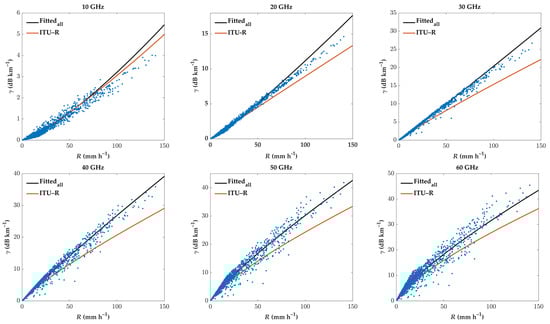
Figure 1. Scatter plots of specific rain-induced attenuation and rain rates at different frequencies. It is worth noting that the rain rates are obtained from an OTT Parsivel disdrometer deployed in Nanjing, whereas the specific rain-induced attenuations are simulated using the T-matrix algorithm based on the DSD data recorded by the disdrometer.