Your browser does not fully support modern features. Please upgrade for a smoother experience.
Please note this is a comparison between Version 1 by Yan Gao and Version 2 by Jessie Wu.
Intelligent fault diagnosis (IFD) plays a vital role in preventative maintenance (PM) for Industry 4.0, which can reduce downtime, improve overall system efficiency, decrease maintenance costs, enhance reliability, and extend the lifespan of machinery, as well as help to optimise operations and make informed decisions. Data-driven approaches based on deep learning (DL) have been widely accepted for IFD in smart manufacturing. Meanwhile, various deep neural network (DNN) architectures have been utilised and developed in the field of IFD.
- intelligent fault diagnosis
- convolutional neural network
- automated machine learning
1. Intelligent Fault DiagnosisD with Traditional Machine Learning
Intelligent fault diagnosis (IFD) methods that can automatically recognise the health states of machines and infrastructures [1][7] are essential for preventative maintenance in Industry 4.0. Many traditional machine learning (ML) approaches can be applied in IFD, such as k-nearest Neighbour (k-NN) [2][8], Naïve Bayes classifier [3][9], support vector machine (SVM) [4][10], decision tree [5][11], and random forests [6][12], etc., which rely on manual features. The pipeline for IFD based on traditional ML can be condensed as shown in Figure 1, which starts from data acquisition through various IoT technologies to feature extraction via handcrafted design and automatic data-driven health state recognition using supervised or unsupervised learning approaches.
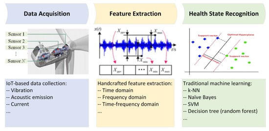
Data for fault diagnosis are usually in time series and collected constantly from different sensors mounted on machines or infrastructures, such as acceleration, displacement, strain, and acoustic signals, as well as ambient conditions like temperature and wind speed. The commonly used features can be categorised into time, frequency, and time–frequency domains based on the extraction methods, e.g., the statistical features, zero-cross rate, wavelet, fractal features in the time domain, discrete Fourier transform (DFT), and power spectral density (PSD) in the frequency domain; energy and entropy from short-term Fourier transform (STFT), wavelet transform (WT), wave packet transform (WPT), and Hilbert–Huang transform (HHT) in the time–frequency domain, as shown in Table 1.
Table 1.
Traditional machine learning pipeline for IFD.
| Machine Learning | Handcrafted Feature Extraction | Approaches |
|---|---|---|
| Traditional ML | Time domain: statistical features, zero-cross rate, wavelet, fractal features, etc. | KNN, SVM, Naïve Bayes classifier, decision tree, random forest, etc. |
| Frequency domain: DFT, PSD, etc. | ||
| Time–frequency domain: STFT, WT, WPT, EMD, HTT, etc. |
2. Intelligent Fault Diagnosis with Deep Learning
2. IFD with Deep Learning
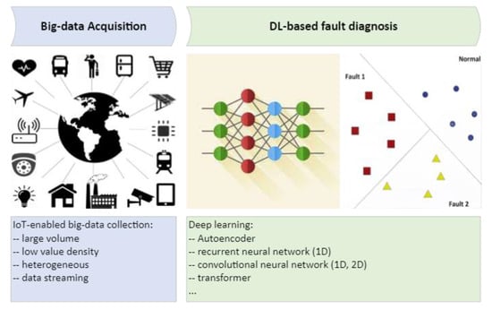
With the rapid development of the IoT, the collected data volume is dramatically higher than ever before and brings more useful information for fault diagnosis. Big data acquisition has four characteristics: volume, quality, variety, and velocity [1][7].
- (1)
-
Volume—the volume of collected data sustainably grows during the long-term operation and maintenance (O&M).
- (2)
-
Quality—a portion of poor-quality data is mingled in the massive data.
- (3)
-
Variety—multi-source data is collected from multiple sources (by different sensors) with a heterogeneous structure.
- (4)
-
Velocity—fast transmission can be enabled in situ via fieldbus cables or at the remote end via high-speed communication like 5G, which promises response and decision-making in near real-time for DT.
Traditional ML relying on handcrafted features becomes inappropriate for big data scenarios. Hence, IFD has been extensively developed based on DL, which can learn features automatically. Its pipeline is shown in Figure 2, consisting of only two steps, i.e., data acquisition and health state recognition, which can accommodate massive data and achieve a higher level of automation by skipping the step of manual feature extraction. The widely used DL approaches for IFD include multilayer perceptron (MLP), autoencoder (AE), recurrent neural network (RNN), convolutional neural network (CNN), transformer, etc.
2.1. Deep LearningL with 1D Time Series
Liu et al. [7][13] and Lu et al. [8][14] employed the stacked sparse AE and the stacked denoising AE for the IFD of bearings, presenting higher diagnosis accuracy than traditional ML methods. Common RNNs, including gated recurrent units (GRUs) and long-term memory networks (LSTM), are theoretically an ideal non-linear time-series forecasting tool and a universal approximator for dynamic systems [9][15]. Ling et al. [10][16] employed RNN to achieve early warning in the fault creep period for nuclear power machinery, together with principal component analysis (PCA), wavelet analysis, and Bayesian inference. Yuan et al. [11][17] utilised LSTM for IFD and remaining useful life (RUL) estimation for aero-engine based on time-series data. Moreover, Neves et al. [12][13][18,19] employed an MLP with train-induced acceleration data to identify the structure health conditions of the KW51 railway bridge. Sajedi and Liang [14][20] proposed a framework based on a fully convolutional encoder–decoder architecture for structural damage diagnosis with the vibration signals from a grid sensor network, which can localise damages and distinguish multiple damage mechanisms with reliable generalisation capacities.
Additionally, 1D-CNN is also inherently suitable for time-series pattern recognition. For example, Wu et al. [15][21] proposed an approach for rub-impact fault diagnosis of a rotor system based on 1D-CNN. Sony et al. [16][22] designed a 1D-CNN to identify multiclass damage using bridge vibration data. 1D CNN was also utilised to detect the change of local structural stiffness and mass based on acceleration from a single sensor [17][18][23,24].
2.2. Deep Learning with 2D Synthetic Images
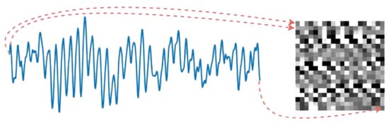
As the monitoring variable for IFD is usually a 1D time series, which is different from 2D images, to leverage the powerful feature learning capability of CNNs, many efforts have been made to transform 1D motion signals into 2D images, including Gramian angular field (GAF) [19][25], wavelet transform [20][21][22][26,27,28], S-transform [23][29], phase space reconstruction [24][30], etc. The GAF, wavelet transform, and S-transform are time-consuming, and the latter two require expert knowledge in the frequency domain for spectrum exploration. In contrast, phase space reconstruction can quickly generate synthetic images with simple backgrounds. For example, time series can be converted through Equation (1) (i.e., min–max normalisation) into a single-channel greyscale image, as shown in Figure 3.
where 𝑃(𝑗,𝑘)∈[0,255] denotes the pixel strength of the grayscale image and j and k are the row and column numbers in the reconstructed image, respectively.
The DL-based IFD can be summarised as shown in Table 2. Previous works [24][25][26][30,31,32] have already proved the effectiveness of using shallow CNNs, like modified LeNet, for IFD. However, they mainly focused on a single sensor and did not consider data fusion for the signals from triple sensors or axes. Meanwhile, the imaging method has not been further developed to generate three-channel images (like RGB) to take advantage of the popular deep CNN architectures.
Table 2.
Deep learning pipeline for IFD.
| Pipeline | Approaches |
|---|---|
| Deep Learning | 1D time series: RNN (including GRU and LSTM), 1D-CNN, etc. |
| 2D synthetic images: (1) Imaging—GAF, wavelet transform, S-transform, phase space reconstruction, etc. (2) Models—shallow single-channel CNNs and classical three-channel deep CNNs via proposed imaging. |
3. Intelligent Fault DiagnosisD with Data Fusion
Data fusion is usually employed in IFD based on multi-sensor data, which is supposed to be an effective way to improve pattern recognition accuracy. It includes data-level and decision-level fusion. Teng et al. [27][33] trained seven individual 1D CNNs using the acceleration signals from the corresponding sensors and fused their classification results at the decision level by hard voting. Compared with data-level fusion, i.e., integrating all acceleration signals into a multi-channel time sequence, decision-level fusion enhanced the classification accuracy by at least 10% in the experiments. However, this comparison consequence is not absolute. For example, Gao et al. [28][34] trained a single 1D CNN with the data-level fused acceleration signals from six sensors on a bridge for structure health-state recognition. Compared with decision-level fusion with hard and soft voting from six individual classifiers, data-level fusion can enhance the test accuracy by more than 20%. Furthermore, Gong et al. [29][35] used multi-channel data-level fusion of time-series signals from different sensors for the IFD of rotating machinery by leveraging CNN-SVM, which also achieves excellent test performance (nearly 100% accuracy). As can be seen, the level of fusion occurrence in IFD is flexible, depending on the used dataset and the selected neural network architecture.