Your browser does not fully support modern features. Please upgrade for a smoother experience.
Please note this is a comparison between Version 1 by Cheng Yang and Version 2 by Jason Zhu.
Distributed generators (DGs) have a high penetration rate in distribution networks (DNs). Understanding their impact on a DN is essential for achieving optimal power flow (OPF). Various DG models, such as stochastic and forecasting models, have been established and are used for OPF. While conventional OPF aims to minimize operational costs or power loss, the “Dual-Carbon” target has led to the inclusion of carbon emission reduction objectives. Additionally, state-of-the-art optimization techniques such as machine learning (ML) are being employed for OPF.
- optimal power flow
- distributed generators
- distribution network
1. Introduction
The proportion of DGs connected to DNs has increased significantly due to the implementation of the “Dual-Carbon” strategy. DGs, which typically consist of photovoltaic cells (PVs) and wind turbines (WTs), offer clean and renewable energy. However, the output from these DGs is often intermittent, resulting in challenges for grid stability. To address these challenges, a battery energy storage system (BESS) is commonly used to smooth out the output curve. The integration of DGs has transformed the traditional DN model from a passive energy receiver into an active network that participates in energy exchange. The energy exchange of DGs is typically achieved through power routers (PRs). OPF is a common technique used to reduce network loss and the cost of DN [1][2][1,2]. The objective of OPF is to minimize system losses and to allocate power rationally among different nodes while ensuring system safety and stability. In addition to these objectives, carbon emissions [3] are also considered as optimization targets.
To achieve OPF with DGs, understanding their impact on DNs is of utmost importance. Ref. [4] investigated the relationship between nodal voltage and the placement of DGs. Two types of DG models, namely stochastic and forecasting, were established to account for their uncertainty. Additionally, the combination of OPF with the electricity market is a hot topic, with recent studies, as seen in references [5][6][7][5,6,7], establishing a demand response (DR) model for calculating locational marginal prices (LMP) and scheduling DG output.
The power flow model, which is the basis of the OPF problem, is also reviewed. The model can be categorized into conventional nonlinear and linear approximation models. The conventional model can reflect the power flow distribution directly, but its nonlinear nature makes it less desirable for calculations. Linear models, on the other hand, can speed up the calculation process but may lose some accuracy. In addition, new component models have been added to the equality and inequality of the model to reflect the new components in DNs.
After defining the basic problem of OPF, various methods for solving the OPF problem are reviewed. However, changes and uncertainties in energy demand, energy flow, and load changes in active distribution networks (ADNs) can lead to voltage offset, frequency dislocation, and power losses at various nodes in the network. As a result, the scheduling and optimization of ADNs can be complex. To address these challenges, it is necessary to optimize the energy distribution and load control of ADNs through an optimal power flow analysis.
Mathematical optimization methods for solving the OPF problem include conventional OPF, Alternating Direction Method of Multipliers (ADMM), Mixed Integer Linear Programming (MILP), Semi-Definite Programming (SDP), Second-Order Conic Programming (SOCP), Quadratic Programming (QP), and others. While mathematical optimization methods can provide rapid convergence and are easy to implement, they may require significant computation resources. The primary concept behind mathematical optimization is to transform the original non-convex OPF model into convex models, thus improving the accuracy and convergence time of the model.
Heuristic optimization methods for solving the OPF problem include Sunflower Optimization (SFO), Particle Swarm Optimization (PSO), Genetic Algorithm (GA), and others. Heuristic optimization methods can handle non-convex and nonlinear problems, but they may not guarantee convergence or optimality and may depend on random factors. These methods reveal the design principles of optimization algorithms by understanding the behavior, function, experience, rules, and mechanisms of action in biological, physical, chemical, social, artistic, and other systems or domains. Under the guidance of specific problem characteristics, the corresponding feature models are refined to design intelligent iterative search-type optimization algorithms.
To the best knowledge of the authors, there is no previous review that extensively covers problem formulation and optimization methods for the OPF problem. Refs. [8][9][10][11][12][13][14][8,9,10,11,12,13,14] have reviewed optimization methods to solve OPF problem, Ref. [12] has reviewed heuristic and conventional algorithms in the DN while introducing some basic principles of OPF; Ref. [8] focused on the mathematical model of OPF, but has not considered other methods or modeling of new models in DN. In their articles, Refs. [13][14][13,14] individually reviewed the ADMM and heuristic methods for OPF. However, it is important to note that these reviews do not encompass the entirety of available optimization methods for OPF. Refs. [9][10][9,10] mainly focused on the problem formulation and the benefits of different methods but only presented a table for the drawbacks without providing a detailed explanation of how the algorithms work. On the other hand, Ref. [11] explained and analyzed some of the methods through case studies but included only a few methods and only in a certain network.
2. Problem Formulation
In general, distribution networks comprise loads, power lines, transformers, and DGs. However, the widespread deployment of DGs such as PV and WT, in addition to the use of various new smart meter technologies, has played a crucial role in transforming distribution networks. As a result, the nature of the distribution network has significantly changed.2.1. Impact of DG in DN
When DGs are connected to DNs, they typically have an impact on nodal voltage and power loss in the network. A comparison of DNs before and after any DGs are connected to the DN is shown in Figure 12 and Figure 23.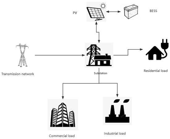
Figure 12.
DN with DGs.
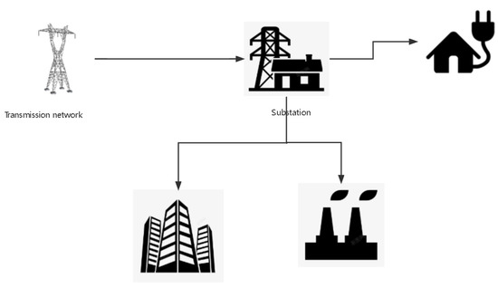
Figure 23.
DN without DGs.
2.2. Generator Modeling
Due to the uncertainty aspect of PVs and WTs, the uncertainty of DGs can be addressed in the following ways: stochastic and forecasting models. A brief summary of the two models is expressed in Figure 34.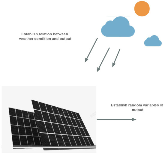
Figure 34.
Brief summary of DG models.
2.2.1. Stochastic Model
The output of DGs is a stochastic event and, hence, can be expressed by a set of random variables. This uncertainty arises from various factors such as weather conditions, load variations, and system disturbances. In their research, Ref. [18] addressed the uncertainty of power outputs of DGs based on probability. They proposed a probabilistic approach to model the output fluctuations of DGs within a certain range. They noted that the output of DGs fluctuates within a range, and thus, they proposed a probabilistic approach to model the uncertainty. Similarly, in their study, Ref. [19] expressed uncertainty via a range of random variables, which were observed over a specified time interval. The goal of these approaches is to effectively capture the uncertainty associated with the output of DGs, thereby supporting the optimization of power system operations. Stochastic models offer several advantages in the evaluation of the reliability and stability aspects of photovoltaic systems. By analyzing probability distributions, these models facilitate the identification and resolution of potential issues. Moreover, they consider uncertainties associated with DGs, effectively incorporating risk factors into system design and planning. This integration enhances the reliability of decision-making processes. Furthermore, stochastic models are particularly well suited for long-term planning purposes. Leveraging historical data, these models can forecast and evaluate future power generation over extended time periods, providing valuable guidance for system design and investment decisions. However, stochastic models also have certain limitations. They heavily rely on the quality and reliability of available data, making them highly dependent on data quality. Insufficient or inaccurate data can adversely impact the accuracy and efficacy of probability models, potentially leading to flawed results and incorrect applications. Furthermore, stochastic models prove inadequate in handling short-term fluctuations and exceptional cases. Due to their inherent characteristics, these models encounter challenges in effectively addressing short-term power generation variations and individual anomalous situations. Consequently, these limitations can introduce forecasting biases and should be carefully considered when utilizing stochastic models in practice.2.2.2. Forecasting Model
Utilizing the relation between weather conditions and output, it is possible to establish a mathematical function to estimate the DG output. Ref. [5] estimated the output of DG by using the weather conditions. The active power output of a PV module was determined based on the input solar irradiance and ambient temperature. The equation was used in the paper to generate an active power curve that corresponds to the solar irradiance and ambient temperature data entered [20]. The commonly used PV power prediction formula calculates the predicted PV power (𝑃𝑉 ) based on weather conditions such as solar radiation intensity (G) and PV panel temperature (T). The formula is as follows:𝑃𝑉(𝑡)=𝐴×𝐺(𝑡)×(1−𝛽×(𝑇(𝑡)−𝑇𝑟𝑒𝑓))
The commonly used wind turbine power prediction formula calculates the predicted wind turbine power P based on weather conditions such as wind speed (V), air density (𝜌), and the rated power of the turbine (𝑃𝑟𝑎𝑡𝑒𝑑). The formula is as follows:
where P represents the predicted wind turbine power, 𝜌 represents air density, A represents the swept area of the turbine blades, 𝐶𝑝
is the power coefficient, and V represents the wind speed.
Forecasting models offer several advantages in the context of DGs. These models leverage advanced algorithms and real-time data to provide accurate short-term predictions, enabling informed decision-making in electricity market operations and real-time dispatch. By considering multiple influencing factors such as weather conditions, seasons, and system parameters, forecasting models enhance the accuracy and reliability of predictions. Additionally, these models support intelligent operation and optimization, providing decision support for power plant operations to optimize generation scheduling and to improve energy utilization efficiency.
However, forecasting models also have certain limitations that should be taken into account. They require high-quality and timely input data to ensure accuracy and reliability. Particularly, accurate weather data and real-time operational data are crucial for achieving optimal performance. Moreover, the establishment and maintenance of high-quality forecasting models involve substantial costs. These costs include the acquisition of extensive data, the implementation of complex algorithms, and the allocation of appropriate computational resources. Therefore, cost-related challenges can arise in the development and maintenance phases. Finally, forecasting models are unable to account for future uncertainties, such as unforeseen weather events. While they provide accurate short-term predictions, unexpected uncertainties in the future cannot be accurately predicted using these models.
𝑃=0.5×𝜌×𝐴×𝐶𝑝×𝑉3
2.3. Demand Response
2.3. Demand Response
DR is a mechanism by which power users receive direct notifications or price increase signals from the power supplier to induce load reduction when the wholesale market price of electricity rises or the system reliability is threatened. This allows users to modify their inherent electricity consumption habits and to reduce or shift their electricity load over a certain period in response to the power supply, ensuring the stability of the power grid and suppressing short-term behavior of electricity price increases. In [5][6][7][5,6,7], the commonly used model for the OPF problem was the electricity elasticity model, which changes the price of electricity for consumers. The article [5] provided an implementation of electricity elasticity in a DR model. The DR model assumes that multiple consumers are connected to each node and that their loads are classified as either flexible or non-flexible. Another approach presented in [6] used electricity prices to build a DR model that modifies the load curve to obtain an equivalent daily load curve. The model considers the elasticity coefficient of the electricity price, which measures the sensitivity of electricity demand to price changes. The elasticity coefficient matrix was used to model user demand response behavior, ensuring that electricity demand in each period is related not only to the current price but also to the electricity price of other periods. This approach is particularly effective when Time-of-Use (TOU) rates are adopted. Finally, the paper [7] proposed a combination of DR and OPF problems, the former being combined with LMP through a Lagrangian function in the latter. This approach optimizes load management by ensuring that LMP reflects the real cost of operating the power system while optimizing the use of flexible loads.2.4. Power Flow Model
Power flow calculations, which involve solving complex equations and handling large-scale networks, often require significant computational time and resources. Ref. [21] introduced a general power flow calculation method for DN with DGs and voltage regulators. The power line can be represented by the 𝜋 model. Transformers can be represented by admittance matrices, while the load can be represented by a vector. The voltage output of a step-voltage regulator can be described using a function of tap, and the impedance and voltage drop of a compensator can be computed using the ratio of the voltage transformer and current transformer and the impedance of the line. A brief summary of the power flow models is expressed in Figure 45.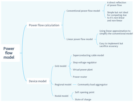
Figure 45.
Brief summary of power flow models.
-
Various models have been proposed from the grid perspective to enhance and optimize power system operations. These models include the superconducting cable model, voltage regulator model, flexible loop converter, and energy router model. Each model serves a specific purpose, such as improving transmission efficiency, voltage regulation, and interconnection between microgrids. In [32], the zero-resistance characteristic of superconducting material was considered, and the superconducting magnet parameters were introduced to reflect the superconducting properties. The modeling of the superconducting cable was constructed using a nonlinear inductance, current source, and leakage resistance to model the cable as an element within the circuit analysis. Voltage regulators play a crucial role in maintaining stable power transmission by adjusting the voltage levels of transformers. These devices ensure that voltage remains within the desired range, mitigating potential issues associated with voltage fluctuations. The power flow calculation method proposed in [21] considers the influence of distributed generation and voltage regulators. The method adds the power equation of distributed generation to the power flow equation of the system and uses the three-phase power injection method in the calculation, which overcomes the convergence problem that traditional power flow calculation methods face. In [33], the modeling of step voltage regulators (svrs) was achieved by assuming that the svr is an ideal component and by modeling it as a three-phase element. The series impedance of the single-phase autotransformer of the svr wes assumed to be zero. The Virtual Power Plant (VPP) model was proposed in [34], which allows for the integration of distributed energy resources as a virtual unit and can participate in the energy market. To interconnect microgrids, power routers must be used. In [35], a stable model for PRs was proposed based on the steady-state power flow calculation model. The line structure in the hybrid AC/DC distribution system based on PR is divided into eight types according to the bus type at both ends of the line and the line type. The power transaction between microgrids relies on energy routers, as proposed by [36]. The energy router is modeled using the port-bus incidence matrix by expressing the energy router using nodal currents and by applying constraints such as Kirchhoff’s current law (KCL) and Kirchhoff’s voltage law (KVL) before embedding it into the existing power system power flow model.
-
The flexible closed-loop converter, constructed using power electronic devices, can achieve DC transmission and can solve the impact of closing AC load loop on the power grid, providing ideas for the closed-loop control of distribution networks. According to [37], there are four operational modes for the flexible closed-loop converter: closed-loop operation mode, power flow transfer mode, circulating current limiting mode, and power flow control mode. The power flow transfer and power flow control modes involve solving the power flow equations. In the power flow transfer mode, when a line of a substation fails or stops operating due to maintenance, the closed-loop controller transfers the remaining load to another line. In the power flow control mode, the closed-loop controller outputs adjustable voltage amplitudes and phases according to the power demand of the secondary power supply line, such as load balancing and minimum line loss, and inserts it into the line for the control of four-quadrant power flow.
-
From the regional perspective, a Community Load Aggregator (CLA) is established. In some studies, a whole residential area is considered to be a node. Ref. [38] established the CLA model by integrating and modeling the residential load, electric vehicle load, and communication load in a community. The model is divided into static and dynamic loads, where static loads refer to the residential and communication loads that have relatively stable characteristics, while dynamic loads refer to the electric vehicle load, which has significant time-varying characteristics and requires optimized scheduling strategies.
-
For a single node, the Soft Opening Point (SOP) model and the State of Charge (SOC) model are established. Ref. [39] modeled SOP and estimated the loss of SOP with the least square estimator. To describe the status of energy storage of a single nodal DG, Ref. [40] used SOC. The formula was used to determine the SOC of a battery based on the battery’s charging and discharging power, charging and discharging efficiency, rated capacity, and calculation time interval.