Laser pulse surface ablation leads to the formation of a crater with a depth of several nanometres up to micrometres. The application of consecutive laser pulses with sequential laser beam movement facilitates the creation of regular laser-formed surface structures, from simple periodical dimples or segments up to polygonal or hierarchical structures ^[1][2][3][4][1,2,3,4]. Such a process of periodical objects laser formation is named laser surface texturing (LST), and it has a wide range of applications: in tribology, material engineering, wettability, brazing, medicine, optics and other areas ^[5][6][7][8][5,6,7,8]. The development of laser surface scanning techniques is needed for increasing the processing rate of LST. Involving the fastest scanning techniques, for example, the application of polygon scanners, acousto-optic beam deflection or sample rotation, has several limitations, such as dead processing time, low deflection angle, sample geometry specification and others. At higher laser surface scanning speeds, it becomes more and more difficult to maintain the high precision of LST, due to the synchronization loop between the laser and the scanning system ^[9][10][11][9,10,11]. The application of high-frequency lasers with ultrashort laser pulses meets the physical limitations of LST, such as heat accumulation between laser pulses and ablated plasma shielding effects ^{[12][13][14][15][16]}[12,13,14,15,16]. The speed limitation for the application of high-frequency lasers becomes important for texturing of 3D bent surfaces ^[17][18][17,18]. There are alternative techniques, such as using low-frequency lasers with high pulse energy for processing entire wide areas at once with a low-speed laser beam or sample movement ^{[19][20][21][22][23][24]}[19,20,21,22,23,24]. For such a technique, plasma shielding and heat accumulation do not have such an important role, but on the other hand, the flexibility and scalability of the laser-processed area is limited by a spot size in comparison with scanning technologies.

The correct choice of an appropriate LST method needs to have an overview of the actual scanning techniques and their limitations. There are a lot of reviews for laser surface scanning strategies for selective melting in 3D printing technology ^[25][26][27][25,26,27]. However, there are no systematic reviews of the existing laser beam scanning strategies for LST with a comparative analysis of their scanning parameters, such as processing rate or maximal scanning speed. In this papentryr, such a review of the classical and recently developed laser surface scanning strategies with a comparative analysis of several scanning parameters of LST is presented. The scanning strategy is defined as a spatial and temporal arrangement of laser paths on the scanning surface, which can be applied in LST.

Different laser surface scanning strategies will be more suitable for different materials, especially considering the laser source limitations [13]. The resulting efficiency, roughness or minimal periodicity of LST structure are significantly influenced by the laser source used. There are a lot of other laser surface processing parameters which significantly affect initiated physical processes of material ablation, such as laser pulse fluence, duration, wavelength, polarization, air pressure or blowing speed or even pulse parity ^{[28][29][30][31][32][33][34][35][36]}[28,29,30,31,32,33,34,35,36].

2. Physical Limitations of Laser Surface Texturing

2.1. Plasma Shielding Effect

The ablation plasma plume spreads over the laser-processed surface, and the next laser pulses will be partially or fully blocked by the plume. The time of the plasma plume surface shielding depends on laser pulse parameters, such as pulse duration, pulse energy or focused spot size. Understanding the main principles of the ablation plasma plume evolution helps in the correct choice of an optimal scanning strategy for LST. The laser pulse absorption initiates the surface temperature reaching the region of overcritical fluid formation ^{[37][38][39][40][41][42][43]}[37,43,44,45,46,47,48]. It was shown that ultrafast solid-to-liquid phase transitions already appear in the first few hundred femtoseconds ^[41][46]. Following this, material expansion is detected in 10–20 picoseconds after laser pulse absorption ^[41][42][46,47]. Exposed materials are able to achieve great speeds, more than 8–10 km/s ^{[44][45][46][47]}[49,50,51,52]. The ablation plume is ejected at the highest speed in the phase explosion regime. The speed of the laser-ablated plume at the very start of the explosion can be described by a kinetic equation of adiabatic expansion ^[48][53]: where 𝑀 is the mass of ablated plume, and 𝐸 is the total energy. In ambient gas, the free expansion of the ablated products will be changed by breaking the movement of the plasma plume with a generation of a frontal shock wave ^[44][48][49][49,53,54]. The following part of the ablated plume has slower medium-size clusters (up to 10,000 atoms) that have ejection velocities of less than 4 km/s and droplets that are slower than 3 km/s ^[44][49]. The pressure in the front shock wave is typically 100–200 atm and decays to close to ambient pressure in 100–200 ns ^[50][55]. In the latter time, the shock wave slows down to the speed of sound and travels forward as a sound wave ^[51][56]. The formation of this shock wave expanding starts in a short time period (0.2–0.5 ns), when the mass of the shock wave becomes comparable with the plume mass ^[52][53][57,58]. The following movement of the plasma plume in ambient gas can be described by the drag model ^[35][51][54][35,56,59]: where 𝑅 is the position of the plasma plume front during expansion, 𝑅0 is the stopping distance of the plume, and 𝛽 is the deceleration coefficient. The stopping position of the ablated plume at normal pressure of ambient gas above the scanned surface is about 1–2 mm and higher ^[35][55][35,60]. The post-ablation products contain clusters and droplets, which continue to have high enough speeds ~100 m/s and inertial mass for achieving bigger distances above the laser-processed surface ^[56][57][61,62]. Such ablation products can cover several centimetres above the processed area for a long time, up to tens of microseconds ^[34][58][34,63]. Plasma and particle shielding effects significantly limit the laser repetition rate and effectiveness of laser surface processing ^[59][64]. The plasma plume transparency dynamic was studied in detail by J. König et al. ^[39][44]. The transparency of the plasma plume above the metallic target was measured by a probe laser beam, which was parallel to the sample surface. It was found that in the first moment of the plasma plume expansion, its transparency decreases down to 10%. The transparency of the plasma plume stays reduced by a certain value till 2–3 µs; during this time, the ablated material expands by hundreds of micrometres ^[35][51][35,56]. Such a highly optically dense plasma plume works as a shield above the processed surface for every subsequent laser pulse, if it comes before the plasma plume dissipates. Overcoming plasma shielding effects can be achieved via the application of a long enough time delay between laser pulses (MHz or lower frequencies), and then the plasma plume optical density becomes low enough before every next laser pulse. Such laser pulse frequencies are applicable for optical systems with laser beam scanning speeds up to 10–20 m/s, which are needed for optimal laser spots overlapping 30–50% ^[10][13][10,13]. An opposite way of overcoming the shielding effects can be achieved via the application of several laser pulses within a short time interval, shorter than that of a plasma plume, which will be expanded above the surface ^[15][60][15,66]. The plasma plume expanding cannot be avoided by the application laser pulse with a short time interval, down to 1–2 ps, but the energy conversion in such fast processes is able to change the ablation mechanism and suppress the shielding effects ^[15][60][15,66]. Such a shielding-suppressing regime is very dependent on processed materials, laser pulse intervals and even pairing of the laser pulses [28]. The frequency of laser pulses for such a mechanism of plasma plume suppression should be in the hundreds of GHz or in THz and can be realized in burst regimes ^{[15][61][62][63][64]}[15,67,68,69,70]. Such a short interval between laser pulses can be achieved with special techniques of pulse dividing, such as crystals array or optical branches ^[28][65][66][28,71,72]. A more practical approach is usually to use long enough time delays when the plasma is gone upon the arrival of the next pulse. Another alternative is application of a scanning strategy with special distribution of laser spots, where the distance between laser spots will be bigger than the plasma plume size (more than 200–300 µm). It can be multibeam surface processing with low frequency of laser pulses or high-speed surface scanning equidistant distribution of laser spots ^[9][67][68][9,73,74]. Several existing scanning techniques of distant laser spot distribution will be discussed in the Section 3 of this revientryw.

2.2. Heat Accumulation in Pulsed Laser Surface Processing

There are a lot of papers in which the important role of heat accumulation during laser surface processing was discussed ^{[69][70][71][72]}[40,75,76,77]. It was shown that in some optimal conditions, heat accumulation becomes a positive factor for increasing the ablation rate or improving the quality of the machined surface ^{[31][73][74][75][76][77][78][79][80]}[31,42,78,79,80,81,82,83,84]. However, undesired high heat accumulation leads to thermal surface degradation with material boiling, intense oxidation and uncontrollable splash formation ^{[69][70][71][81][82][83]}[40,75,76,85,86,87]. The evaluation of the heat accumulation level can be performed by thermal field modelling or by experimental ^{[32][71][82][84][85][86]}[32,76,86,88,89,90]. After ablation, a thin remelted layer with a number of point defects and dislocations, produced by ultrafast cooling and shock wave, remains in the laser spot area ^[87][88][91,92]. The output laser-irradiated surface will be contaminated by precipitation of the ablated products and associated oxidation of the upper surface layers ^{[89][90][91][92]}[93,94,95,96]. In most cases, the surface ablation process has a semi-thermal character (𝑘𝐵𝑇𝑖≥𝜀𝑏). For example, at Gaussian distribution of energy in the laser spot, the laser pulse residual heat stays in the subsurface layers and in the near-ablated zone. The residual heat in subsurface layers can be brought by secondary effects: heat conductivity from ablated layers, ballistic and diffusion effects, convective and radiating energy exchange between the ambient and solid target, and shock wave spreading ^{[37][44][89][93][94]}[37,49,93,97,98]. These residual effects have a great influence on the quality and efficiency of LST in a high-repetition multi-pulse regime ^[31][71][95][31,76,99]. Of course, even a single laser pulse can produce many thermal effects: material boiling, oxidation and splash formation. These thermal effects have short-term character, and in the biggest cases, high-temperature fields dissipate within 2–5 µs ^[71][96][41,76]. However, in the case of multi-pulse laser surface processing, the residual heat is rising from pulse to pulse in the laser-affected zone. Such heat accumulation is able to prolong and intensify the thermal processes to an undesired level, although this occurs in the case whereby one single pulse is unable to initiate significant thermal processes. The value of heat accumulation can be predicted theoretically as a sum of the residual heat from all laser pulses in a laser pulse sequence ^[69][96][40,41]: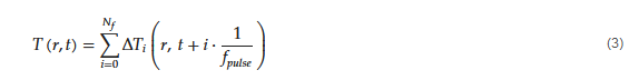 where 𝑇(𝑟,𝑡) is the temperature in the point 𝑟 at the time moment 𝑡, 𝑁𝑓 is the full number of the laser pulses in the pulse sequence, ∆𝑇𝑖 is the residual temperature after 𝑖-th laser pulse and 𝑓𝑝𝑢𝑙𝑠𝑒 is the laser pulse generation frequency. In this equation, the residual temperature ∆𝑇𝑖 after absorption of a discrete laser pulse can be approximately defined from a 3D model with an instance heat point source ^[96][97][98][41,100,101]. A more detailed study of the heat accumulation effects under moving Gaussian laser spots was conducted by Bauer et al. ^[69][40]. For evaluation of heat accumulation under a laser-scanned surface in a fixed subsurface point, a semi-planar thermal model can be applied ^[71][99][76,102]: 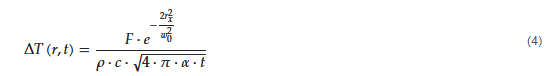where 𝑥 is the coordinate of a fixed surface point, 𝑟𝑥 is the distance from the centre of the laser spot to the fixed surface point 𝑥, 𝛼 is the thermal diffusivity, 𝜌 is the material density and 𝑐 is the specific heat. It has been found that the maximal heat accumulation in a thin subsurface layer is achieved within a specific time interval when the laser beam central point has already passed the fixed subsurface point ^[71][99]. In the exemplary work of F. Bauer et al. ^[69], the critical temperature for heat accumulation was defined through experiments involving offset temperature shifting in the laser-scanned surface. The defined offset temperature shift was compared with the corresponding temperature shift in thermal simulations. It was shown that the critical temperature for heat accumulation in steel surface processing has a value near 607 °C. Oxidation and surface degradation were detected at higher temperatures of the scanned surface preheating, even when other laser scanning parameters were not changed ^[69][71]. is the specific heat. It has been found that the maximal heat accumulation in a thin subsurface layer is achieved within a specific time interval when the laser beam central point has already passed the fixed subsurface point [76,102]. In the exemplary work of F. Bauer et al. [40], the critical temperature for heat accumulation was defined through experiments involving offset temperature shifting in the laser-scanned surface. The defined offset temperature shift was compared with the corresponding temperature shift in thermal simulations. It was shown that the critical temperature for heat accumulation in steel surface processing has a value near 607 °C. Oxidation and surface degradation were detected at higher temperatures of the scanned surface preheating, even when other laser scanning parameters were not changed [40,76]. The correct choice of scanning strategy and optimization of laser beam parameters brings the possibility to overcome the aforementioned physical limitations, especially heat accumulation. The next development of the IR in-process fast measurements will be in on-fly control of the laser beam parameters during laser surface scanning. The on-fly IR control of the laser surface processing in combination with high-speed scanning technique is a way to achieve the high standards of Industry 4.0.

3. Scanning Techniques of LST

The need for increasing the throughput of LST technologies stimulates the development of new strategies for high-speed laser surface processing. There are several well-known scanning technologies for high-speed laser beam deflection: galvo scanners, polygon scanners, piezo scanners, static and resonant scanners, micro-lens scanners, electro-optic deflectors (EOD) and acousto-optic deflectors (AOD) ^{[21][100][101]}[21,103,126]. The inertial scanning systems have a maximal deflection angle and a number of resolvable spots on the scanned surface ^[101][126]. There are two traditional techniques for high-speed laser surface machining with a large processing area: galvanometer beam scanning and polygon optical scanning systems ^[102][103][127,128]. The maximal scanning speed of the available galvanometer scanners lies in the range of 10–40 m/s, whereas the polygon scanner is able to achieve a scanning speed of more than 1000 m/s ^{[102][104][105]}[127,129,130]. The higher speed of the polygon scanners is of great benefit in the fast provision of LST in large areas. However, polygon scanners do not provide the smooth wall profiles of vector scans for cutting a circumference or trepanning large holes greater than 50–150 µm. The laser beam deflection in polygon scanners should be corrected by an additional galvanometer scanner. For LST, when the processed area is smaller than 15% of the working field, the polygon scanners are not cost-efficient, and alternative techniques will be more suitable ^[102][127]. The correct choice of scanning strategy helps to improve the laser-processed surface quality and precision of the laser pulse delivery. The output processing rate of LST depends on a favourable choice of the combination of the scanning strategy with different scanning techniques (Table 1, rows 1 and 2). The maximal processing rate of 9000 cm²/min for DLIP was found by a team from Fraunhofer Institute IWS ^{[106][107][108][109]}[131,132,133,134]. The period and distribution of laser surface textured objects with DLIP are directly dependent on the wavelength of the laser beam ^[110][135]. This limitation makes it difficult to apply the DLIP for texturing surfaces in cases of irregular structure or complex nonsymmetrical textures, for example, for super hydrophilic surfaces, high optical absorbance and hydrodynamic effects. The process of the formation of such a structure is based on self-organized effects, cone-like structure formation or programmable direct laser machining with spot size resolution ^{[111][112][113]}[136,137,138]. For the laser-controlled formation of fine complex submicron structures, a combination of the DLIP technique with dynamic systems has been provided. The processing rate of such a technique is about 0.7–10 cm²/min ^[107][114][132,139]. The benefit of such a combination of DLIP with regular micro-texturing techniques gives the possibility to create unique hierarchical structures ^[107][115][132,140]. Submicron surface structures might be created by laser scanning with the self-organized formation of LIPSS ^[116][117][116,141]. In this case, the laser scanning parameters, such as laser spot overlapping and scanning speed, have a key role for highly regular LIPSS (Table 1, rows 3 and 16). The achieved processing rate for LIPSS formation directly depends on the applied scanning speed. For example, I. Gnilitskyi et al. ^[118][142] have reported a processing rate of LIPSS forming on stainless steel equal to 6.3 cm²/min with a scanning speed of 3 m/s. The last study predicts several times higher processing rates with polygon scanners ^[72][77]. LIPSS forming is competitive with industrial standards of nano-manufacturing (~1 cm² in 10 s) ^[119][143]. Like the DILP technique, LIPSS might be applied for the formation of hierarchical surface structures in combination with micro-texturing. The benefit of such a solution is that the period of the upper LIPSS can be smaller than half of the laser wavelength ^[119][143]. Another highly productive LST strategy is via forming an array of micro-objects by dividing the laser beam with diffraction or shadow masks ^{[120][121][122][123]}[144,145,146,147] (Table 1, rows 12 and 17). This scanning strategy could be used in cases when the pulse energy is high enough to be divided into multi-beams ^[86][90]. The distance between laser spots is given by mask parameters or diffraction light distribution. In the case of the application of a solid-state static mask, the spot distance is constant, and part of the laser beam energy will be lost. The application of spatial light modulators (SLMs) gives us the possibility to change the laser spot distribution of the scanning process, but the average power will be limited to under 300 W ^[124][148]. However, a processing rate of up to 1800–5400 cm²/min in a multibeam scanning solution can be achieved ^[124][125][148,149]. LST by straight hatch lines is the most suitable strategy for the polygon scanner technology (Table 1, rows 13–16, 20, 22). In this case, the laser beam scanning speed achieves high values, up to 800–2000 m/s ^[73][42]. The polygon scanner has a throughput several times higher in comparison to galvanometer scanners ^[126][150]. However, providing LST with a polygon scanner needs to involve a correlation between mirror position and laser pulse generation for the precise formation of micro-objects. This imposes a restriction on the scanning speed for LST. The maximal processing rates up to 7680 cm²/min were achieved for a linear texture, and this was performed at 320 m/s ^[72][77]. However, for polygon scanners, the problem of processing arrays of micro-objects with specific geometry remains unresolved ^[127][151]. It is difficult to control the laser drilling of micro-objects with high-speed scanning, because there are substantial data in relation to large arrays with small objects or micro-objects, up to 800 MB per second ^[105][130]. Additionally, there is not enough time for precise control of laser spot distribution inside every micro-object in the array. Moreover, ultra-high-speed laser beam processing with polygon scanning involves artefacts such as jitter, banding, bow and other problems characteristic of these systems. These artefacts involve two components: periodical and random. There are several hardware techniques for reducing polygon scanner artefacts, but known classic methods of laser beam processing of the array of objects in ultra-fast scanning systems do not have a fully finished solution to the mentioned problems, and scanning techniques must still be improved ^[127][128][151,152]. The galvanometer scanner can create curved lines purposefully with the fast swinging of two deflection mirrors. This technique was applied in direct laser formation of an array of micro-objects with different structures (Table 1, rows 6–11). The galvanometer scanner is able to achieve a processing rate of up to 428 cm²/min for forming an array of micro-objects with a one-beam simple scanning technique at one pulse per object ^[129][153]. The high precision formation of surface structures with hatch filling of more complex micro-objects reduces the processing rate to 25 cm²/min ^[130][38]. Noticeably higher processing rates with galvanometer scanners might be achieved by splitting the laser beam into several spots. In this case, a processing rate of up to 5400 cm²/min is reached ^[124][148]. A multibeam solution has potential for industrial applications, especially where there is a need to create a wide array of periodical surface microstructures ^[116][124][116,148].