Your browser does not fully support modern features. Please upgrade for a smoother experience.
Please note this is a comparison between Version 1 by Alisson Marques Silva and Version 2 by Camila Xu.
Virtual screening (VS) is an in silico technique used in the drug discovery process. During VS, large databases of molecular structures are automatically evaluated using computational methods. With the use of VS, it is expected to identify molecules more susceptible to binding to the molecular target, typically a protein or enzyme receptor.
- drug discovery
- virtual screening
- machine learning
- deep learning
1. Introduction
The discovery and manufacturing processes for new drugs have been in constant evolution in the last decade, with benefits and results directly related to the life quality improvement of the world population [1]. The effectiveness of the production and manufacturing strategies is increasing, although the costs involved remain a challenge [2]. The development of a new drug has an average cost between 1 and 2 billion USD and could take 10 to 17 years, from target discovery to drug registration [3]. These costs reflect a time-consuming, laborious, and expensive process, which implies drugs with high added value and, often, of restricted acquisition, at least for a third of the world’s population [4][5][4,5].
In addition, part of these costs are related to a low success rate, with only 5% of phase I clinical trial drugs entering the market [6]. These impacts are even more significant in places such as Asia and Africa, where more than 50% of the population lives in poverty or with a lower average income than in the rest of the world [4][7][4,7]. The conditions that restrict the access of this fraction of the population to essential medicines contribute to the increase in the mortality of tens of thousands of people every year, 18 million of which could be avoided if these medicines became accessible [8].
One way to reduce drug discovery and manufacturing limitations, minimizing cost and time impacts, is by using computer-aided drug design (CADD), also known as molecular modeling. In such an approach, the design stages and analysis of drugs are carried out through a cyclic-assisted process entirely conducted through in silico simulations. These simulation techniques can evaluate essential factors in drug discovery, such as toxicity, activity, biological activity, and bioavailability, even before carrying out in vitro and in vivo clinical trials [9]. An initial step of the CADD approach is screening virtual compound libraries, known as virtual screening (VS). VS is a molecule classification method that exploits biological or chemical properties available in large datasets. The International Union of Pure and Applied Chemistry (IUPAC) defines VS as computational methods that classify molecules in a database according to their ability to present biological properties against a given molecular target [10].
Popular VS techniques originated in the 1980s, but the VS word first appeared in a 1997 publication [11]. In the early 1990s, the rapid evolution of computers created the hope that companies could accelerate the discovery process of new drugs. These computing advances have enabled several advances in combinatorial chemistry and high-throughput screening (HTS) technologies, allowing for vast libraries of compounds to be synthesized and screened in short periods. The VS process aims to choose an appropriate set of compounds, removing inappropriate structures and limiting the use of a significant number of resources. In this way, identifying hits with computational methods proved to be a promising approach because, even before carrying out the biological assays, computational simulations could indicate which compounds were most likely to be good hits.
2. Virtual Screening
VS is an in silico technique used in the drug discovery process [12][13][14][15][16][12,13,14,15,16]. During VS, large databases of molecular structures are automatically evaluated using computational methods. With the use of VS, it is expected to identify molecules more susceptible to binding to the molecular target, typically a protein or enzyme receptor.
VS works like a filter (Figure 1), eliminating more molecules so that the number of final candidate molecules that may become a drug is much smaller than the initial number. In Figure 1, molecules that can become a good drug are initially selected because they have properties that favor their action or are similar to drugs with known functioning. Candidate ligands are then analyzed, and molecules in which pharmacophoric groups that indicate the likelihood of toxicity are identified are eliminated. In the next step, the best poses for candidate ligands are identified. During this VS process, the candidate ligands can have their compositions and structures readjusted to enhance their properties; mainly, their pharmacokinetic characteristics (absorption, distribution, metabolism, excretion, and toxicity (ADMET)). It may require new cycles of optimizations in the composition and structure of candidate ligands. This way, the ligands are prepared for biological assays after this process.
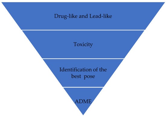
Figure 1.
Virtual screening process.
Furthermore, the VS allows for the selection of compounds in a database of structures with a greater probability of presenting biological activity against a target of interest. VS can also eliminate compounds that may be toxic or that have unfavorable specific pharmacodynamic and pharmacokinetic properties. In this sense, biological assays should be performed only with the most promising molecules, leading to a lower cost and shorter development time [13].
There are essentially three main approaches of VS: structure-based VS (SBVS), ligand-based VS (LBVS), and fragment-based VS (FBVS). The following sections detail these approaches.
2.1. Structure-Based Virtual Screening
SBVS, also known as target-based VS (TBVS), attempts to predict the best binding orientation of two molecules to form a stable complex. The SBVS technique encompasses methods that explore the molecular target’s 3D structure. SBVS is the preferred method when the 3D structure of the molecular target has been experimentally characterized [14]. SBVS tries to predict the likelihood of coupling between candidate ligands and target protein, considering the binding strength of the complex. The most used SBVS technique is molecular anchoring due to the low computational cost and the satisfactory results [15][16][15,16].
Molecular docking emerged in the 1980s when Kuntz et al. [17] developed an algorithm that explored the geometrically feasible docking of a ligand and target. They showed that structures close to the correct ones could be obtained after docking. This technique tries to predict the best position and orientation of a ligand in a binding site of a molecular target so that both form a stable complex. To this end, it uses the structural and chemical complementarity resulting from the interaction between a ligand and a molecular target through scoring functions, often complemented with pharmacophoric restrictions [18]. SBVS is often used with proteins and enzymes as receptors, but it can also be used in other structures, such as carbohydrates and DNA. However, although the approach was promising, it was only in the 1990s that it became widely used, when there was an improvement in the techniques used in conjunction with an increase in computational power and greater access to the structural data of target molecules.
The use of SBVS has advantages and disadvantages. Among the benefits are the following: (a) there is a decrease in the time and cost of screening millions of small molecules; (b) there is no need for the physical existence of the molecule, so it can be tested in silico before being synthesized, (c) there are several tools available to assist SBVS.
As a disadvantage of using SBVS, it can be highlighted that (a) some tools work best in specific cases but not in more general cases [19]; (b) it is difficult to accurately predict the correct binding position and classification of compounds due to the difficulty of parameterizing the complexity of ligand–receptor binding interactions; (c) it can generate false positives and false negatives.
Despite the disadvantages noted above, many studies using SBVS have been developed in recent years [12][20][21][22][23][24][25][12,20,21,22,23,24,25], which shows that although SBVS has weaknesses, it is still widely used for designing new drugs due to the reduction in time and cost.
2.2. Ligand-Based Virtual Screening
LBVS uses ligands with known biological activity aiming to identify molecules with similar structures using virtual libraries of compounds. In this approach, the molecular target structure is not considered. Instead, it follows the principle that structurally similar molecules may exhibit comparable biological activity. Thus, LBVS tries to identify compounds with similar molecular scaffolds or pharmacophore moieties, increasing the chance of finding biologically active compounds.
LBVS is performed by comparing the descriptors or characteristics of known molecules derived from reference compounds and compared with the descriptors of the molecules of the databases. For this purpose, similarity measures are used. There are several ways to verify the similarity between two sets of molecular characteristics, but the Tanimoto coefficient [26] is one of the most used to perform this task [27].
One of the most common LBVS classifications techniques is the number of dimensions of the represented descriptor (1D, 2D, or 3D):
-
1D descriptors cover molecular properties such as weight, number of hydrogen-bond donor and acceptor groups, number of rotatable bonds, number and atoms type, and computed physicochemical properties, such as logP and water solubility (log D), degree of ionization, and others;
-
2D descriptors are those based on molecular topology. Therefore, they are built based on the molecular connectivity of the compounds. Two-dimensional descriptors can exist as structural descriptors and topological indices [28]; structural descriptors are those characterizing the molecule by its chemical substructure. They can be represented in 2D graphs or binary vectors. For example, the number of aromatic rings in a molecule, the connectivity index, and the Carbo index (which calculates molecular similarity) are 2D descriptors. Topological indices define the molecule’s structure according to its shape and size. Simpler indices characterize the molecules according to their size, shape, and degree of branching, and more complex indices consider both the properties of the atoms and their connectivity;
-
3D descriptors provide molecular information in the context of the spatial distribution of atoms, molecular properties, or chemical groups. 3D descriptors need to consider molecular conformations, meaning they need to consider the spatial distribution of particles, molecular properties, or chemical groups [29]. Studies have demonstrated that a single descriptor does not perform better than another for all VS [30]. Therefore, the molecules are, in most cases, described as a set of descriptors. Examples of 3D descriptors are the electrostatic potential and van der Walls.
LBVS is more suitable for use in the following situations: (a) whenever there is little information about the structure of the molecular target. In addition, it is used to enrich the database for SBVS experiments; (b) for targets with large amounts of experimental data available or where the drug-binding site is not well defined, LBVS methods are generally superior to SBVS methods [31]; (c) the simultaneous use of the LBVS and SBVS approaches can increase the accuracy of the VS, as the LBVS can eliminate some false-positive compounds identified as promising by the SBVS technique, increasing the chances of obtaining good results [11].
The LBVS technique has the following limitations: (a) the currently available LBVS techniques have not yet shown the desired performance, but the prediction accuracy is expected to increase rapidly in the coming years [14][20][14,20]; (b) minor chemical modifications in similar molecules can either potentiate an activity or make it inactive [32]. Wermuth [33] shows how relatively modest changes in a molecule with known biological activity can lead to compounds with very different activity profiles. This is known as activity cliffs [34]. In this way, a molecule identified by the LBVS technique as similar to another with known activity may be inactive, leading to a false-positive result.
2.3. Fragment-Based Virtual Screening
FBVS has also been a powerful approach to finding early hits that can lead development [35]. FBVS aims to test fragments of low-molecular-weight molecules against macromolecular targets of interest [36]. FBVS usually generates a candidate compound from a chemical fragment with low molecular weight (generally less than 300 Da), low binding affinity, and simple chemical structures [37]. These compounds are then used as starting points for drug development. However, due to their low molecular weight, fragment hits are generally weak binders and need to be made into larger molecules that bind more tightly to the target to be made into a lead. Therefore, the methods used in FBVS and the fragment binding modes are critical in fragment-based screening [35][37][35,37].
Over the last 20 years, FBVS using nuclear magnetic resonance (NMR) has been a prominent approach. FVBS has made it possible to obtain a high success rate with increased development speed and decreased cost of producing new drugs [36]. Moreover, there is no need for intervention by medicinal chemists in the early stages of increasing fragment molecules and their transformation into molecules with more significant biological activity. Several FBVS approaches have been used today, and the development of the ligand from a fragment using ML has gained prominence [38].
The main advantage of using FBVS is the low complexity of the fragments used in the simulation [35], which allows for the use of different techniques (which have pros and cons that must be analyzed according to the situation) for the development of new compounds and cost reduction in drug development [35].
3. Virtual Screening Algorithms
VS has become a widely used strategy for drug discovery, and as seen in the previous section, it can be classified into SBVS, FBVS, and LBVS. Moreover, VS techniques can be divided according to the algorithms used to perform its pipeline.
In the literature, several taxonomies are used to classify the algorithms, such as those presented in [39][40][41][42][43][44][39,40,41,42,43,44]. However, due to the diversity of the algorithms described here, researchers chose to use a new taxonomy, as shown in Figure 2, in which the algorithms are divided into similarity, quantitative, machine learning, meta-heuristic, and others.
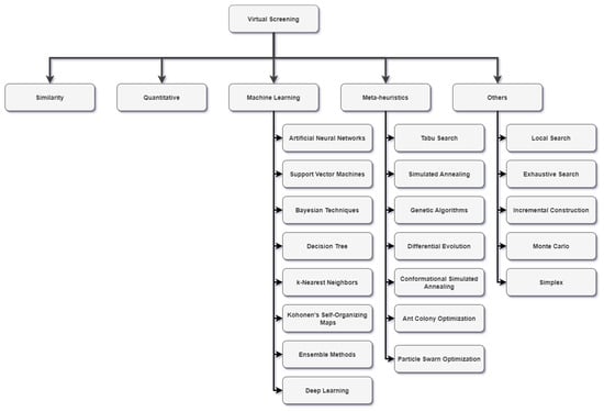
Figure 2.
VS algorithms taxonomy.
3.1. Similarity-Based Algorithms
In similarity-based approaches, algorithms assume that a molecule with a similar structure to another whose biological activity is known may share similar activity [16]. In a similarity search, a structure with a known biological activity relating to the target is used as a reference. These reference structures are then compared to a database of known molecules so that the similarity between them is determined. This similarity can be determined by a coefficient of similarity applied to all molecules in the database. However, two highly similar compounds may have different biological activities. Thus, small changes in a molecule can either generate an active or an inactive compound [27]. The methods based on similarity tend to only require a few pieces of reference information to create predictive models [45]. Therefore, their simplicity and effectiveness have made them widely accepted by the scientific community. Additionally, the similarity-based algorithms can be combined with other methods such as ML, meta-heuristics, and others to improve the results.
The similarity-based algorithms can be divided into 2D, 3D, quantum, and hybrid approaches. The 2D approaches are the most intuitive VS technique based on the 2D similarity of substructures compared to various 2D descriptors using a similarity coefficient [46][47][48][46,47,48]. Then, in 3D approaches, the similarity search can also be performed through 3D molecular representations, such as in pharmacochemical [27][32][33][49][27,32,33,49], overlapping volumes [50][51][50,51], and molecular interaction fields (MIFs) [16]. Next, the quantum approach mainly focuses on quantum descriptors that produce good results but depend on conformation [52][53][54][55][52,53,54,55]. Finally, this could still be achieved with a hybrid approach [56][57][58][59][60][61][56,57,58,59,60,61] using more than one of the options above.
3.2. Quantitative Algorithms
QSAR modeling is one of the well-developed LBDD methods. QSAR models have attempted to predict the property and/or activity of interest of a given molecule.
A QSAR model is formed by a mathematical equation that compares the characteristics of the investigated molecules with their biological activities. Mathematically, according to Faulon and Bender [62], any QSAR method can usually be defined as the application of mathematical and statistical methods to the problem of finding empirical equations in the form Yi = F (X1, X2, …, Xn), where the variable Yi is the approximate biological activity (or another property of interest) of the molecules and X1, X2, …, Xn are structural experimental or calculated properties (molecular descriptors such as molar weight, logP, fragments, number of atoms and/or bonds). F is some mathematical relationship empirically determined that must be applied to descriptors to calculate property values for all molecules.
At first, QSAR modeling was only used with simple regression methods and limited congener compounds. However, QSAR models have grown, diversified, and evolved to modeling and VS in large databases using various ML techniques [63].
Benedetti and Fanelli [64] show several commonly used QSAR models (local, pharmacophore-based, and global QSAR models). Fan et al. [65] used a ligand-based 3D QSAR model based on in vitro antagonistic activity data against adenosine receptor 2A (A2A). The resulting models, obtained from 268 chemically diverse compounds, were used to test 1897 chemically distinct drugs, simulating the real-world challenge of a safety screening when presented with novel chemistry and a limited training set. Additionally, it presented an in-depth analysis of the appropriate use and interpretation of pharmacophore-based 3D QSAR models for safety.
The objective of a QSAR model is to establish a trend of molecular descriptor values that correlate with the values of biological activity [17]. Therefore, it is essential to minimize the prediction error, for example, by using the sum of squared differences or the sum of absolute values of the differences between the expected and observed activities in Yi for a training set. However, before constructing the model, the data need to be pre-processed and adequately prepared to build and validate the models [62].
3.3. Machine Learning-Based Algorithms
The availability of large databases of molecules storing information such as the structure and biological activity makes it possible to use predictive models based on ML, which require a large amount of data from active and inactive compounds to make the prediction. Therefore, ML techniques have been increasingly used in VS due to their accuracy, expansion of chemical libraries, new molecular descriptors, and similarity search techniques [45].
ML is a field of artificial intelligence and computer science devoted to understanding and building algorithms that learn based on data, analogy, and experience [37]. The ML algorithms use datasets to learn and, based on knowledge acquired in the learning process, make decisions, make previsions, and recognize patterns. In addition, it is expected that the overall performance of the ML system will improve over time and the system will adapt to changes [41].
ML techniques stand out due to their ability to learn from data (examples). Furthermore, the learning methods can be divided into supervised, unsupervised, or reinforcement, depending on the algorithm [66]. Supervised learning requires a training set in which each sample is composed of the input and its desired output, i.e., the learning algorithm uses labeled data [67]. In supervised learning, the system parameters are adjusted by the error between the system output and the desired output [39]. In unsupervised learning, the training set is composed only of the inputs. The desired output is not available or does not exist at all [67]. The objective of unsupervised learning is to construct the system knowledge based on the spatial organization of the inputs. In other words, unsupervised learning aims to discover patterns using unlabeled data. Reinforcement learning uses a mechanism based on trial-and-error and reward, in which the correct action awards the learner and the wrong actions punish them [68]. The learner decides on actions based on the current environmental state and the feedback from previous actions [69]. The learner has no prior knowledge of what action to take, and the aim is to find the actions that maximize long-term reinforcement. Reinforcement learning is often used in intelligent agents [41].
The power of VS is increased with ML because it makes it possible, instead of performing computationally costly simulations or exhaustive similarity searches, to track predicted hits much faster and more accurately [23][70][71][23,70,71]. ML is used to find new drugs, repositioning compounds, predict interactions between ligands and protein, discover drug efficacy, ensure safety biomarkers, and optimize the bioactivity of molecules, to mention a few [72]. It can be seen in Figure 2 that the ML algorithms can be divided into artificial neural networks (ANNs), support vector machines (SVMs), Bayesian techniques, decision trees (DTs), k-nearest neighbors (k-NN), Kohonen self-organized maps (SOMs), deep learning (DL), and ensemble methods. The following sub-sections explain the ML algorithms, show how they can be used, and contribute to the drug discovery process.
3.3.1. Artificial Neural Networks
ANNs are mathematical models inspired by the processing capacity of the human brain. A neural network is composed of a set of computational units called neurons, which are a simple mathematical model of biological neurons [67]. The neurons are connected through synaptic weights, which simulate the strengths of synaptic connections of the biological brain [73]. The synaptic weights represent the knowledge in the ANNs, and the learning is performed by changing these weights. Generally, the ANNs use a supervised learning algorithm to update the weights based on errors obtained between the network output and the desired output. The neural network structure can be defined by the number of layers, the number and type of neurons, and the learning algorithm [74]. For example, Figure 3 illustrates the structure of a neural network with two inputs, four neurons in the first layer (hidden layer), one neuron in the second layer (output layer), and the synaptic weights [75].
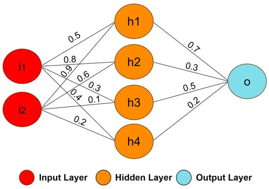
Figure 3. An example of a simple neural network model. The model was formed by two inputs (i1 and i2), four neurons (h1, h2, h3, and h4) in the first layer, one neuron (o) in the output layer, and the synaptic weights.
Different efforts introduce ANNs in medicinal chemistry to classify compounds, principally in studies with QSAR, to identify potential targets and the localization of structural and functional characteristics of biopolymers. In such a context, Lobanov [76] introduces a review to argue how ANNs can be used in the VS pipeline from combinatorial libraries, showing how selecting descriptors is essential to evaluate the ANNs. Furthermore, in such a review it is emphasized that descriptors can be found in one-dimensional (1D), two-dimensional (2D), and three-dimensional (3D) forms and can be used to create a model for ADMET properties profiles.
Tayarani et al. [77] propose an ANN model based on molecular descriptors to obtain the binding energy using the physical and chemical descriptions of the selected drugs. The authors showed a high correlation between the observed and calculated binding energies by the ANN since the average error ratio was less than 1%. The experimental results suggested that ANN is a powerful tool for predicting the binding energy in the drug design process. Recently, Mandlik, Bejugam, and Singh [78] wrote a book chapter to show the possibilities of using ANNs to aid in developing new drugs.
3.3.2. Support Vector Machine (SVM)-Based Techniques
SVM is a supervised ML algorithm for classification and regression tasks [41][79][41,79]. In a D-dimensional data space, an SVM creates a hyperplane (h) or a set of hyperplanes to cluster input data elements according to the similarity expressed in the descriptors’ characteristics. Such hyperplanes employ linear and nonlinear functions to identify margins that separate a set of classes (x). In general, the greater the operating margin, the lower the classifier’s generalization error. Intuitively, a good separation is achieved using the hyperplane with the most significant distance looked at in the closest training data of any class. For example, Figure 4 shows a classification instance where x1 and x2 denote a pair of classes, with h1, h2, and h3 as operating margins in which h1 does not separate the classes, h2 separates the classes, and h3 separates them with the highest operating margin.
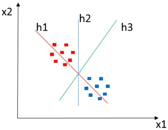
Figure 4. Classification example using SVM. The red and blue squares represent objects of each class to be classified. h1 does not separate classes. h2 does, but only by a small margin. h3 manages to separate them with the maximum margin.
SVMs have recently been cited as a promising technique for VS [79][80][81][82][79,80,81,82]. Rodrígues-Pérez et al. [77] describe how the algorithm can be used in VS and create a comparison with others in ML presenting its advantages and disadvantages. As an example, it is mentioned that SVM has evolved as one of the “premier” ML approaches and has been used as a approach of choice, given its typically high performance in compound classification and property predictions on the basis of limited training data. This is possible thanks to the adaptability and versatility of SVM for specialized applications.
Silva et al. [83] used Autodock Vina in the docking process, but they proposed an alternative SVM-based scoring function. They showed that while Autodock Vina offers a prediction of acceptable accuracy for most targets, classification using SVM was better, which illustrates the potential of using SVM-based protocols in VS. Finally, Li et al. [84] describe the ID-Score, a new scoring function based on a set of descriptors related to 2278 protein–ligand complexes extracted from Protein Data Bank (PDB). The results indicated that ID-Score performed consistently, implying that it can be applied across a wide range of biological target types.
3.3.3. Bayesian Techniques
Bayesian techniques are based on Bayes’ theorem and describe the probability of an event occurring due to two or more causes. This approach combines previous beliefs with new evidence to compose a hypothesis and describe a model. The main implementation of this model was algorithms such as the naïve Bayes classifier and Bayesian networks [85].
In repositioning and drug discovery scenarios, the Bayesian algorithms identify the probability of a compound possessing biological activity for a specific target. Therefore, Bayesian techniques can be used, for instance, to find novel active scaffolds against the same target or to find compounds that are more active or that possess improved ADMET properties when compared to the main structure [86]. However, Bayesian networks were not explicitly superior to much simpler approaches, based, for example, on the Tanimoto coefficient [87].
3.3.4. Decision Trees
DTs are a supervised ML algorithm that describes functions to take data attributes as input and return a single output, sometimes called a “decision” by some authors [69]. DTs make decisions by performing a sequence of tests, starting in the first tree node called “root” and proceeding in a top–down strategy until reaching the last level of the structure, with nodes typically named leaves.
To compose the aforementioned structure as a tree, firstly, a test value that reports some relationship with each input attribute is associated with each internal node, except the root. Then, such nodes are labeled with the attribute’s decision possibilities, and leaves specify the final results that the function should return according to the characterizations exploited. Figure 5 shows how a DT works. In Figure 5 diagram, a toy example is introduced to identify whether the weather is good for playing sports outdoors. The decision process starts in the root node where weather (i.e., sunny, cloudy, or rainy) is observed. Then, according to weather conditions, the decision function estimates a novel specific node (at a lower level), repeating this process until some leaf is achieved, which is used to extract and return the result.
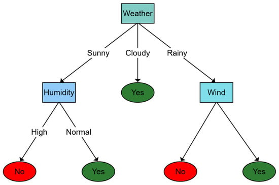
Figure 5. Classification example using a decision tree to determine whether the weather is good enough to go outside. The first level is determined by how the weather is. Depending on the answer, a new question is selected, or the answer is found. For example, if the weather is sunny, it is questioned about the humidity depending on whether it is high or normal to determine whether the final answer is yes or no.
Lavecchia [76], argue that DTs are a useful alternative to creating combinatorial libraries to predict the similarities between drugs or specific biological activities. However, to extract high performance using DTs, a single tree structure is not enough. In this context, some efforts, such as those presented in [88], propose applying a set of DTs to increase the forecast variation. These proposals are called random decision forests (RDFs). This generalization of DTs is employed by Lavecchia to demonstrate improving the LBVS performance, the predictive ability of quantitative models, and unique decision tree algorithms. Considering reseaourchers' paper’s focus, decision-making forests can be considered as a choice to determine protein-binding affinity, in addition to being widely used in other coupling applications. In DT, molecules can be classified from the input data employed to design their structure during the training stage [70].
Considering VS, is possible to observe DTs employed as a support tool and classifier functions. An alternative method to construct DT-based classifiers with higher precision for repositioning and discovery of drugs, improving accuracy as its structure grows in complexity, has been described by Ho and collaborators. The proposed method uses a pseudorandom procedure to choose a member of a resource vector. According to the choice made, DTs are generated using only the components that have the selected characteristics [89]. DTs have been applied to investigate interactions among biological activities, chemical substructures, and phenotypic effects [88]. This study assumes chemical structure fingerprints provided by the PubChem system, divided across four assays according to biological activity data in a 10-fold cross-validation (CV) sensitivity, specificity, and Matthews correlation coefficient (MCC) with results of 57.2~80.5%, 97.3~99.0%, and 0.4~0.5, respectively.
3.3.5. K-Nearest Neighbors
KNN is the most popular unsupervised learning method used for classification and regression, whose strategy boils down to looking for, from some prefixed data input element, the k-closest neighbors. In scenarios where input data elements are fashioned by the same descriptors and drawn in the same n-Dimensional space, some metrics can be chosen to compare them, including those based on distances such as Euclidean, cosine, and Manhattan [90]. In a correlation analysis context, Pearson [91] and Kendall [92] may be sufficient. For input data elements represented by a particular structure such as trees, Resnik [93], Jiang [94], and Lin [95] should be considered.
Once the adequate metric is found, the param K in the KNN algorithm should be defined before execution, which matches the number of neighborhood points extracted as results. For example, if k = 1, only the training element closest to the instance to be classified is selected. If k = 5, the five elements closest to the instance are selected, and based on the classes of the five elements, the class of the test element is inferred. The idea of this algorithm is that the class to which a compound belongs can be defined by the class to which the closest neighbors belong (more similar compounds, for example), considering weighted similarities between the compound and its closest neighbors [96].
In VS, Shen et al. [97] created a new drug design strategy that uses KNN to validate developed QSAR models. They identified and synthesized nine potential anticonvulsant drugs by evaluating a library of more than 250,000 molecules. Of these, seven were confirmed as bioactive (a success rate of 77%). Peterson et al. [98] used KNN in QSAR and VS studies and found 47 types I geranyl transferase inhibitors in a database with 9,500,000 chemicals. Seven were successfully tested in vitro and presented activity at the micromolar level. These new hits could not be identified using traditional similarity search methods that demonstrate that KNN models are promising and can be used as an efficient VS method.
3.3.6. Kohonen’s SOMs
Kohonen’s self-organizing maps (SOMs) [99] are unsupervised algorithms that use competitive networks formed by a two-layered structure of neurons. The first layer is called the input layer, with its neurons completely interconnected to the neurons of the second layer, which is organized in a dependent arrangement of the object to be mapped. Kohonen maps are therefore formed by connected nodes with an associated vector corresponding to the map’s input data (e.g., molecular descriptors). Kohonen algorithms can analyze grouped data to discover multidimensional structures and patterns. The Kohonen networks can also be considered an unsupervised neural network since having a known target vector is not necessary. It is considered a self-organized algorithm since it can decrease the size of a data group while maintaining the real representation concerning the relevant properties of the input vectors, resulting in a set of characteristics of the input space.
The Kohonen self-organizing maps are defined by Ferreira et al. [100] as competitive neural networks with a high degree of interconnection between their neurons that can form mappings, preserving the topology between the input and output spaces. For example, in VS, Kohonen’s SOMs could be employed extensively in drug repositioning and scaffold hopping [101]. Noeske et al. [102] used Kohonen’s SOMs to discover new targets for metabotropic glutamate receptor antagonists (mGluR). Experiments have revealed distinct subclusters of mGluR antagonists, and localization overlaps with ligands known to bind to histamine (H1R), dopamine (D2R), and various other targets. These interactions were later confirmed experimentally and exhibited significant binding affinities between the predicted mGluR antagonists for the targets. This led to a mGluR1 antagonist and selective subtype (Ki = 24 nM) based on a coumarin scaffold. This compound was later developed into a series of leads.
In another study, Noeske et al. [103] used Kohonen’s SOMs to map the drug-like chemical space using pharmacophore descriptors. The experiments demonstrated that other G protein-coupled receptors (GPCRs) could interact with mGluR ligands (mGluR1: dopamine D2 and D3 receptors, histamine H1 receptor, mACh receptor; mGluR5: histamine H1 receptor). Lastly, the results were experimentally confirmed, and their IC50 ranged from 5 to 100 μM. Hristozov et al. [104] use Kohonen’s SOMs in LBVS to rule out compounds with a low probability of having biological activity. The proposed idea can be used, according to the authors, (1) to improve the recovery of potentially active compounds; (2) to discard compounds that are unlikely to have a specific biological activity; and (3) to select potentially active compounds from a large dataset. In a recent paper, Palos et al. [105] applied Kohonen’s SOMs in ligand clustering to perform drug repositioning in FDA-approved drugs. This research suggests that four FDA drugs could be used for Trypanosoma cruzi infections.
3.3.7. Ensemble Methods
Ensemble methods combine multiple models rather than employing a single model to increase model accuracy. The results are significantly more accurate when the combined models are used. This has increased the popularity of ensemble methods in ML [106].
Sequential and parallel ensemble techniques are the two main types of ensemble methods. Adaptive boosting (AdaBoost) is an example of a sequential ensemble technique that generates base learners in a sequence. The sequential generation of base learners facilitates the base learners’ dependence on one another. The model’s performance is then improved by giving previously misrepresented learners more weight.
Base learners are generated in parallel ensemble techniques, such as a random forest. To foster independence among base learners, parallel methods use the parallel generation of base learners. The application of averages results in a significant reduction in error due to the independence of base learners.
Most ensemble methods employ a single algorithm in base learning, resulting in uniformity among all base learners. Homogeneous base learners are base learners of the same type and share many of the same characteristics. Heterogeneous ensembles are created when heterogeneous base learners are used in other approaches. Different types of learners make up heterogeneous base learners.
In a recently published paper, Helguera [107] reported that using ensemble techniques, such as bagging [108] and boosting [109], provides better predictions than any of the above techniques in isolation in ML. Therefore, Helguera proposed an ensemble method based on genetic algorithms (GAs). To investigate potential Parkinson’s disease therapeutics, Helguera applied his proposed method for the LBVS of dual-target A2A adenosine receptor antagonists and MAO-B inhibitors. Finally, he showed that the ensemble method outperformed individual models.
A combination of VS and MD with Ensemble methods to evaluate the ∆Tm is described in [110], which used Ensemble methods to estimate the ∆Tm experimental values of DNA intercalating agents. These authors also evaluated three docking methodologies, and the best five molecules were submitted to MD simulations.
3.3.8. Deep Learning
DL is a large class of ML techniques based on neural networks in which inputs are successively transformed into alternative representations that better allow for pattern extraction [39][41][42][43][44][67][69][73][111][39,41,42,43,44,67,69,73,111]. The word “deep” refers to the fact that circuits are typically organized in many layers, meaning that the computation paths from inputs to outputs have many steps. DL is currently the most widely used approach for applications such as visual object recognition, machine translation, speech recognition, speech synthesis, and image synthesis; it also plays a significant role in reinforcement learning applications. Figure 6 shows the main difference between ANNs and the DL approach, namely the number of hidden layers. In ANNs, one or two hidden layers are usually used, while in DL, more than five layers are used, leading to more meaningful processing and better results.
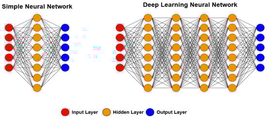
Figure 6. Differences between ANN and DL architectures. In a simple neural network, one or two hidden layers are used, while in DL, more than two layers are always used. With this, the required processing is more significant; however, in most cases, the results are better.
Several studies with DL have been applied in VS. Multiple reviews [63][112][113][114][115][63,112,113,114,115] have presented a detailed explanation of DL and how it can be used in VS and described methods and techniques along with problems and challenges in the area. Bahi et al. [116] present a compound classification method based on a deep neural network for VS (DNN-VS) using the Spark-H2O platform to label small molecules from large databases. Experimental results have shown that the proposed approach outperforms state-of-the-art ML techniques with an overall accuracy of more than 99%.
Joshi et al. [117] used DL to create a predictive model for VS, and the molecular dynamics (MD) of natural compounds against the severe acute respiratory syndrome coronavirus 2 (SARS-CoV-2) were deployed on the Selleck database containing 1611 natural compounds for VS. From 1611 compounds, only four compounds were found with drug-like properties, and three were non-toxic. The results of MD simulations showed that two compounds, Palmatine and Sauchinone, formed a stable complex with the molecular target. This study suggests that the identified natural compounds may be considered for therapeutic development against SARS-CoV-2.
More recently, Schneider et al. [118] presented DL for VS in antibodies to predict antibody–antigen binding for antigens with no known antibody binders. As a result, the DL approach for antibody screening (DLAB) can improve antibody–antigen docking and structure-based VS of antibody drug candidates. Additionally, DLAB enables improved pose ranking for antibody docking experiments and the selection of antibody–antigen pairings for which accurate poses are generated and correctly ranked.
3.4. Meta-Heuristic Algorithms
Meta-heuristic approaches are widely applied in searching for and finding approximate optimum solutions. Meta-heuristic can be classified as single-solution or population-based [119]. Single-solution meta-heuristics aim to change and improve the performance of a single solution. Tabu search (Section 3Section 3.4.1.4.1.) and simulated annealing (Section 3Section 3.4.2.4.2.) are examples of single-solution meta-heuristics used in drug discovery. On the other hand, population-based methods maintain and improve multiple solutions, each corresponding to a unique point in the search space [120]. Population-based meta-heuristics applied in drug discovery include genetic algorithms (Section 3Section 3.4.3.4.3.), differential evolution (Section 3Section 3.4.4.4.4.), conformational space annealing (Section 3.4.5.), ant colony optimization (Section 3Section 3.4.6.4.6.), and particle swarm optimization (Section 3Section 3.4.7.4.7.).
3.4.1. Tabu Search
The TS algorithm performs the search using a memory structure that accepts the investigation of movements that do not improve the current solution [121]. In TS, the memory is used to create a Tabu list consisting of solutions that will not be revisited, preventing cycles, making it possible to explore unvisited regions, and improving the decision-making process through past experiences.
PRO_LEADS [122] is one of the most popular algorithms using TS in VS. It proposes using a TS algorithm to explore the large search space and uses an empirical scoring function that estimates the binding affinities to order the possible solutions. PRO_LEADS was tested on 50 protein–ligand complexes and accurately predicted the binding mode of 86% of the complexes.
3.4.2. Simulated Annealing (SA)
Simulated annealing, a general probabilistic meta-heuristic, is a method that can approximate the global optimum of a given function given ample search space [123]. In summary, SA is an approach for resolving bound-constrained and unconstrained optimization issues. This method simulates the actual physical procedure of heating a material and gradually lowering the temperature to reduce defects and reduce system energy.
A new point is generated randomly during each iteration of the simulated annealing algorithm. A probability distribution with a temperature-dependent scale is the foundation for the new point’s distance from the current point or the scope of the search. All new points that lower the objective are accepted by the algorithm, as are points that raise the objective with a certain probability. The algorithm can look globally for more potential solutions rather than becoming stuck in local minima by accepting points that raise the goal. An annealing schedule is chosen to lower the temperature as the algorithm progresses. The algorithm reduces the scope of its search to a minimum to converge as the temperature drops.
Within the MD context, simulated annealing molecular dynamics (SAMD) involves heating a particular crystallographic (ligand–receptor) complex to high temperature, followed by gradual slow cooling to unveil conformers of reasonable energy minima [124]. The process is usually repeated over multiple cycles (10–100) [124][125][124,125]. One use of SAMD is calculating the optimal docked pose/conformation for a particular ligand within a specific binding pocket, as in the CDOCKER docking engine. Hatmal and Taha [126] use a methodology implemented to develop pharmacophores for acetylcholinesterase and protein kinase C-θ. The resulting models were validated by receiver-operating characteristic analysis and in vitro bioassay. Thus, in this research, four new protein kinase C-θ inhibitors among captured hits, two of which exhibited nanomolar potencies, were identified.
3.4.3. Genetic Algorithms
GAs are a technique for tackling both obliged and unconstrained improvement issues that depend on regular choice, the interaction that drives natural development [127]. They are implemented as a computer simulation where a population undergoes mutations to find better solutions. Each new individual represents a possible solution to the problem. For each new generation, the most suitable individuals are evaluated. This process selects some individuals for the next generation, and they are recombined and mutated to generate new individuals. Although random, they are targeted to a better solution by exploring available information to find new search points where better performance is expected. This process is repeated until it is finalized. The problem with GAs is that they typically have a poor processing time. Therefore, they are mostly used in challenging problems.
GAs are widely used in VS. For example, Bhaskar et al. [128] used a genetic algorithm in their docking process to uncover 14 lead candidates that selectively inhibit the NorA efflux pump competing with its substrates. In addition, Rohilla, Khare, and Tyagi [129] evaluated, using a genetic algorithm, the ability of the IdeR transcription factor (essential in regulating the intracellular levels of iron) to bind to the DNA after being exposed to some compounds. The most potent inhibitors showed IC50 values of 9.4 mM and 6.9 mM. After analyzing the inhibition results, it was possible to find an important scaffold in inhibiting the protein (benzo-thiazol benzene sulfonic).
Xia et al. [130] applied a genetic algorithm to investigate a potential therapy to treat neurodegenerative disorders (e.g., Parkinson’s disease) and stroke. They performed a VS experiment based on the X-ray structure of the Pgk1/terazosin complex and selected 13 potential anti-apoptotic agents selected from the Specs chemical library. In vitro experiments performed by the authors demonstrated a high chance of three of the selected compounds binding to hPgk1-like terazosin. These results indicate that they can act by activating hPgk1 and as apoptosis inhibitors.
3.4.4. Differential Evolution
DE is a heuristic strategy for globally optimizing nonlinear and non-differentiable continuous space functions. A broader group of evolutionary computing algorithms includes the DE algorithm. The DE algorithm begins with an initial population of candidate solutions, just like other popular direct search strategies such as GAs and evolution strategies. Then, by introducing mutations into the population, these candidate solutions are iteratively improved, keeping the fittest candidate solutions with lower objective function values. The basic idea of this operation is to add a randomly selected individual to the difference between two other randomly selected individuals [131].
MolDock [132] combines DE with a cavity prediction algorithm. In a VS test of ligands against target proteins, MolDock identified the correct binding mode of 87% of the complexes. This result was better than Glide [133], Gold [134], Surflex [135], and Flexx [136] in similar databases.
3.4.5. Conformational Space Annealing (CSA)
CSA is a stochastic global search optimization algorithm that uses randomness in the search process. Due to this, this method works well for nonlinear objective functions where other local search algorithms do not. It utilizes global optimization to find the optimal solution for a given objective function satisfying for any. CSA can be considered a type of GA because it performs genetic operations while maintaining a conformational population [137]. Here, the terminologies of “conformation” and “solution” are used interchangeably. CSA contains two essential ingredients of Monte Carlo and SA.
As in Monte Carlo, CSA only works with locally minimized conformations. However, in SA, annealing is performed in terms of temperature, while in CSA, annealing is performed in an abstract conformational space while the diversity of the population is actively controlled.
The CSA performance is described in Shin [138], which evaluates two existing docking programs, GOLD [139] and AutoDock [140], on the Astex diverse set.
3.4.6. Ant Colony Optimization
ACO is an algorithm inspired by the behavior of ants in the search of food. One of the central ideas of ACO, proposed by Dorigo et al. [141], is the indirect communication based on trails (or paths) of pheromones between a colony of agents called ants. In nature, ants search for food by walking on random tracks until they find it. Then, they return to the colony and leave behind a trail of pheromones. When other ants find this trail, they stop following random tracks and follow the trail to obtain food and return to the colony. Over time, the pheromone evaporates, reducing the ants’ attraction to a certain path. The more ants go through a path, the more time it takes for the pheromone to evaporate. Pheromone evaporation is important because it prevents an optimal local solution from becoming excessively attractive over time.
The Protein–Ligand ANT System (PLANTS) [142] is used in protein–ligand docking. In this algorithm, an artificial colony of ants is used to find the conformation of the least energized ligand at the binding site. In this artificial colony, the behavior of real ants is imitated by marking the low-energy conformations with pheromone trails. This information of the pheromone track is then modified in the subsequent iterations, aiming to increase the probability of generating conformations with lower energy. According to Reddy et al. [143], this algorithm behaves well when tested with GOLD in experimentally developed structures.
3.4.7. Particle Swarm Optimization
Particle swarm optimization (PSO) optimizes a problem iteratively by improving a candidate solution respecting a certain quality measure. It has many similarities to GAs. In PSO, the system is initialized with an individual (population) representing random solutions, and it searches for the best solution by updating the generations. In the PSO, the possible solutions are called particles and fly through the problem space following the current optimal particles. Comparing it with GA, PSO is easier to implement because it has fewer parameters to calibrate. Although classified as an evolutionary algorithm, PSO does not have the survival characteristic of the fittest or the use of genetic operators, such as crossing and mutation [144].
Liu, Li, and Ma [145] compared a PSO algorithm against four state-of-the-art docking tools (GOLD, DOCK, FlexX, and AutoDock with Lamarckian GA) and it performed better in the evaluated database. Gowthaman, Lyskov, Karanicolas [146], and PSOVina [147] are other examples of particle swarming applied in VS.