Your browser does not fully support modern features. Please upgrade for a smoother experience.
Submitted Successfully!
 +1 credit
Thank you for your contribution! You can also upload a video entry or images related to this topic.
For video creation, please contact our Academic Video Service.
| Version | Summary | Created by | Modification | Content Size | Created at | Operation |
|---|---|---|---|---|---|---|
| 1 | Xavier Escaler | -- | 4278 | 2024-02-29 14:33:33 | | | |
| 2 | Catherine Yang | Meta information modification | 4278 | 2024-03-01 01:40:45 | | |
Video Upload Options
We provide professional Academic Video Service to translate complex research into visually appealing presentations. Would you like to try it?
Cite
If you have any further questions, please contact Encyclopedia Editorial Office.
Fernández-Osete, I.; Bermejo, D.; Ayneto-Gubert, X.; Escaler, X. Acoustic Emissions in Crack Detection. Encyclopedia. Available online: https://encyclopedia.pub/entry/55740 (accessed on 23 June 2026).
Fernández-Osete I, Bermejo D, Ayneto-Gubert X, Escaler X. Acoustic Emissions in Crack Detection. Encyclopedia. Available at: https://encyclopedia.pub/entry/55740. Accessed June 23, 2026.
Fernández-Osete, Ismael, David Bermejo, Xavier Ayneto-Gubert, Xavier Escaler. "Acoustic Emissions in Crack Detection" Encyclopedia, https://encyclopedia.pub/entry/55740 (accessed June 23, 2026).
Fernández-Osete, I., Bermejo, D., Ayneto-Gubert, X., & Escaler, X. (2024, February 29). Acoustic Emissions in Crack Detection. In Encyclopedia. https://encyclopedia.pub/entry/55740
Fernández-Osete, Ismael, et al. "Acoustic Emissions in Crack Detection." Encyclopedia. Web. 29 February, 2024.
Copy Citation
Acoustic emissions (AE) are becoming an important tool for hydraulic turbine failure detection and troubleshooting. In particular, artificial intelligence is a promising signal analysis research hotspot, and it has a great potential in the condition monitoring of hydraulic turbines using acoustic emissions as a key factor in the digitalisation process.
acoustic emission
crack propagation
crack initiation
fatigue damage
condition monitoring
1. Acoustic Emission
The phenomenon of AE was first observed as audible sounds when materials were deformed. Already in the eighth century, the Arabian alchemist Jabir ibn Hayyan (also known as Gerber) wrote that Jupiter (tin) gives off a “harsh sound” or “crashing noise”, referring to an audible emission produced by the twinning of pure tin during its plastic deformation. Gerber also described that Mars (iron) makes a louder sound during forging. This sound was produced by the formation of martensite during the cooling process [1]. Joseph Kaiser conducted the first comprehensive study into the phenomena of AE [2]. The most significant discovery of Kaiser’s work was the irreversibility phenomenon that now bears his name, the Kaiser effect: if a material is loaded, it will emit some AE signals, but if it is unloaded and later reloaded, it will not emit any AE signal until the maximum charge level from before is reached. AEs are currently used in many areas of research, quality control and industry in general. AEs have been used in the study of different materials: metals [3][4][5][6][7][8], composites [9][10], additive manufactured materials [11] and human and other living being tissues [12][13]. Other applications are real-time leak detection and localisation [14][15], tool-wear monitoring and other studies on machining processes [16][17][18][19], the health monitoring of large structures [20][21], the study of cavitation and its erosion and the monitoring of fatigue crack onset and growth.
The elastic waves produced by an AE propagate inside the material and can be captured using a suitable sensor attached on the surface at the time the waves reach the surface. A contact type sensor is normally used in AE measurements, such as the one shown in Figure 1a. In most of the cases, a piezoelectric crystal enclosed inside a protective housing is employed as an AE transducer. These sensors are exclusively based on the piezoelectric effect out of lead zirconate titanate (PZT). AE signals are detected in the form of dynamic motions over the surface of a material, and they are converted into electrical signals using a PZT piezoelectric transducer [22]. In contrast to accelerometers, the frequency response function (FRF) of a PZT AE sensor presents a significant deviation from a preferred flat frequency response due to the proximity between the PZT natural frequencies and the characteristic elastic wave frequencies. Thus, the sensitivity of an AE sensor depends on the frequency. Additionally, unlike accelerometers, which are carefully designed to measure only the motion component parallel to their axis, AE sensors respond to motions in any direction [23]. Figure 1b shows the FRF of an AE sensor. Sensors of different models have different FRFs. Consequently, if different AE signals are to be compared, they shall be measured with the same sensor model.
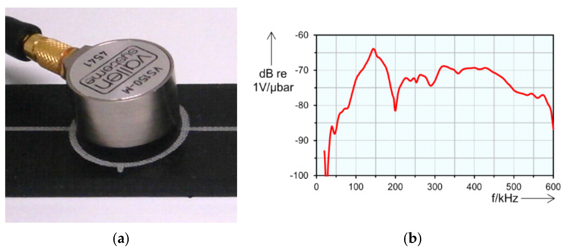
Figure 1. AE sensor Vallen VS150-M: (a) sensor picture; (b) frequency response function [24].
Typical data acquisition schemes for AE measurements comprise both amplification and filtering stages. Amplifiers boost the signal voltage to bring it to a level that is optimal for the measurement stage. Along with several stages of amplification, frequency filters are incorporated into the AE measurement chain. These filters define the frequency range to be used and attenuate low frequency background noise. This process of amplification and filtering is called “signal conditioning”. It “cleans” the signal and prepares it for processing. After conditioning, the signal is digitalised for its recording or/and processing. Sampling frequencies must be very high (of the order of MHz) because of the high frequencies of AE signals [22].
AE signals can be classified into two general classes: burst signals and continuous signals. Burst signals have a clearly defined start and end relative to background noise, and thus, they have a well-defined duration (Figure 2a). A burst signal, from its beginning to its end, is also called a hit. On the other hand, continuous signals, although they present variations in their amplitude and frequency over time, do not have a defined beginning and end, and they are maintained as long as the process that generates them is active (Figure 2b).
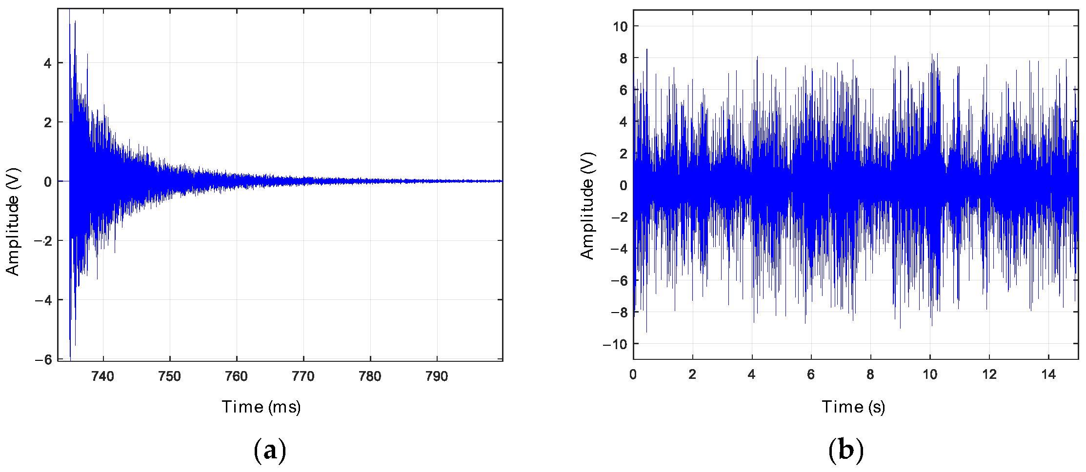
Figure 2. AE signals: (a) burst signal or hit; (b) continuous signal.
Approaches for analysing AE signals can be divided in two groups: parameter-based analysis and signal-based analysis. In the first approach, as the signal is acquired, the characteristic parameters that describe the waveforms of the different parts of the signal (hits) are computed, and even the whole hit can be recorded; thus, parameter-based analysis can be used with burst signals only. This is usually an on-line processing. In a signal-based analysis approach, the raw signal is usually recorded for further analysis. It can be used with burst and continuous signals [22].
1.1. Parameter-Based Analysis
Burst signals have to be clearly defined relative to the background noise. In order to detect burst signals, it is necessary to have previously set a threshold amplitude level above the background noise. In Figure 3, the main parameters of a characteristic AE time-response signal are presented. The burst signal onset is defined as the instant at which the absolute voltage exceeds the predetermined threshold level. It is considered that the burst signal has ended when a determined time, called the Hit Lockout Time, has passed without any further signal crossing the threshold [25]. The burst signal from its onset to its end is called a hit.
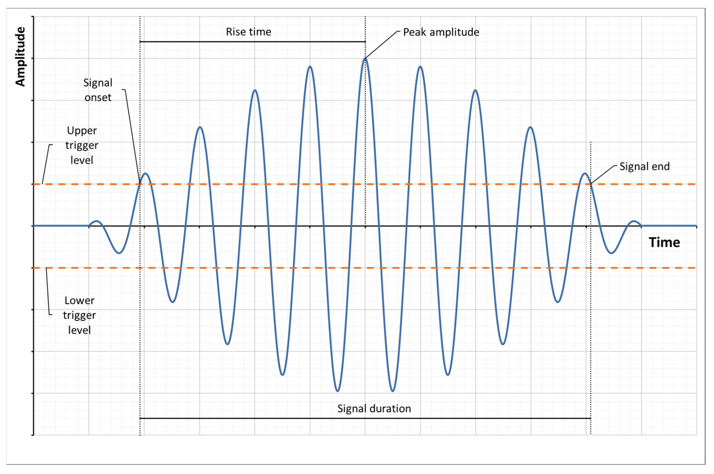
Figure 3. Definition of the AE parameters on a hypothetical signal.
Parameter analysis is based in the extraction of descriptors that contain most of the waveform information, which are the following ones (Figure 3) [25]:
-
Counts are the number of times within the signal that the AE amplitude reaches the threshold level. For example, this number is 7 in Figure 3.
-
Amplitude is the peak voltage of the signal waveform, which can be positive or negative. Amplitudes are expressed in decibels on a logarithmic scale. Commonly, 1 μV is defined as 0 dB AE.
-
Energy is generally defined as a Measured Area under the Rectified Signal Envelope (MARSE). While this is an “engineering” value, another definition of energy, known as “absolute energy”, is computed as the integration of the rectified squared waveform. It is considered analogous to the actual energy released from the AE source:

Duration is the time interval between the first count and the last descending threshold crossing.
Some parameters can be calculated from the hit-frequency spectrum. The most remarkable ones are the peak frequency and the centroid frequency:
-
The peak frequency is the frequency corresponding to the highest magnitude in the spectrum.
-
The centroid frequency is given by the following expression:

1.2. Signal-Based Analysis
In this subsection, several approaches that consider the entire AE waveform are described. The basic premise is that the AE waveforms are recorded, and their changes over time are characterised and interpreted [26]. Different analyses can be conducted, such as those presented in the following subsections.
1.2.1. Frequency Analysis
Frequency analysis techniques are widely used, ranging from simple filtering to more sophisticated approaches. AE signals can be filtered with a high-pass filter in order to remove the low-frequency background noise [26]. Furthermore, signals can be demodulated using the Hilbert transform [27], such as in cavitation analyses, in order to identify the characteristic frequencies of its dynamic behaviour [28].
1.2.2. Time–Frequency Analysis
This family of techniques is well suited for non-stationary signals and includes the wavelet transform (WT) and the short-time Fourier transform (STFT). An advantage of these techniques is that they are able to relate changes in the frequency characteristics of the signal within the time domain [26]. Both techniques can also be used as a signal conditioning stage to improve denoising. These transforms produce tri-axis diagrams (X-time, Y-frequency and Z-amplitude) that are plotted in colour-scaled plots called spectrograms.
Although the WT shows a good performance for processing signals in the time–frequency domain, its application requires the selection of a suitable wavelet function before the analysis. As different wavelet functions result in different output results, the Empirical Mode Decomposition (EMD) method was introduced in 1998 [29] to reduce the impact of a pre-defined wavelet function. EMD decomposes any complex dataset into a finite number of Intrinsic Mode Functions (IMFs) that provide information about instantaneous frequency and energy instead of the global pictures defined by the Fourier spectral analysis [30][31]. Enhanced Empirical Mode Decomposition (EEMD) is a refinement of EMD used to overcome a mode-mixing problem that appears with intermittent components [32]. In EEMD, the mode-mixing problem is removed by adding white noise to the processed signal. Lei et al. [33] have compared decomposed signals using both methods and concluding that EEMD is more accurate than EMD. Complete EEMD (CEEMD) is a further refinement wherein the decomposition provides a more accurate reconstruction of the original data [34].
1.2.3. Machine Learning Approaches
Pattern recognition and clustering have been proposed to discriminate different types of AE events. The goal is that waveforms with similar features are grouped (or clustered), corresponding to different source mechanisms or failure types. A set of characteristics, or parameters, are deducted from each type of signal, which is then considered by the algorithm to determine the clusters. Different machine learning algorithms are used with AE signals. The k-nearest neighbour algorithm (k-NN) is one of the simplest ones: the output value of any test point is the average of the k-nearest output values from the training distribution [26]. The random decision forest (RF) is an ensemble learning algorithm for regression problems that constructs a robust number of decision trees during training, and the average prediction value of the training trees is returned as the final predicted result [35]. The support vector machine (SVM) is an algorithm that constructs a hyperplane with the shortest possible distance between it and the sample points. It has exhibited a good generalisation capability and high prediction accuracy in cases of limited training datasets [36].
Neural networks (NNs) consist of an input and output layers that are connected through a number of hidden layers, all mathematically related via non-linear relationships that must be estimated (learning) [25]. Convolutional neural networks (CNNs) are defined as NNs that use the convolutional operation, which is defined as the dot product between a grid-structured set of numbers (weights) and similar grid-structured inputs drawn from different spatial locations in the input [37]. CNNs are commonly used in image recognition processes. For example, Gaisser et al. [38] employed spectrograms of AE signals measured in hydraulic turbines as the input of a CNN to detect cavitation.
2. Crack Detection Using Acoustic Emissions
Fatigue cracks are one of the predominant failure modes in hydraulic turbines. Fatigue damage starts with the initiation of cracks and continues with their propagation until an unstable size is reached that produces the breakdown of the component. AEs can be used to track this process of crack initiation and growth.
Dunegan et al. [39] presented a model that states that the cumulative AE counts (η) on a specimen in a tensile strength test are proportional to the fourth power of the stress intensity factor (K), as expressed by Equation (3):

In spite of that, some tests presented with aluminium and beryllium specimens in the same study exhibited a mechanical behaviour that differed significantly from the one predicted by the model, with experimental exponents higher than four.
Bassim [40] presented a relationship between the AE count rate (𝑑𝜂/𝑑𝑁) and the stress intensity factor range (Δ𝐾) in metallic materials, as expressed by Equation (4):
 where 𝑁 is the number of fatigue cycles, Δ𝐾 is the stress intensity factor range, and 𝐵 and 𝑝 are material-dependent constants. This expression is similar to the Paris–Erdogan law [41], which, when combined with Equation (4), permits the derivation of a relationship between fatigue crack growth rate (𝑑𝑎/𝑑𝑁)) and 𝑑𝜂/𝑑𝑁 for metallic materials, as given by Equation (5) [42][43][44]:
 where a is the fatigue crack length, and m and s are material-dependent constants. This means that a can be estimated through the integration of 𝑑𝜂/𝑑𝑁, and a can be estimated without knowing the load-time history or complex calculations of 𝐾. Roberts et al. [42] performed fatigue tests on specimens made from grade S275JR steel, with load ratios R of 0.1, 0.3 and 0.5 and the simultaneous measurement of AEs. Measuring only the counts among the top 10% of the applied range, they claimed that the prediction based on the above procedure exhibited a reasonably close correlation with the experimental results.
Yu et al. [45] developed a model that includes the acoustic energy rate, crack driving forces, fracture toughness and load ratio, as expressed in Equation (6):
 where 𝑑𝑈/𝑑𝑁 is the absolute energy change rate (based on AE data), 𝑅 is the load ratio, 𝐾𝑐 is the fracture toughness, 𝐾𝑚𝑎𝑥 is the high-stress intensity factor, and 𝑞2 and 𝐷2 are material-dependent constants.
Li et al. [46] developed a methodology for AE crack sizing based on bending tests on rail steel specimens for different load conditions. A classification index based on the wavelet power (WP) of the AE signal was first established to distinguish the crack closure-induced AE waves from the crack propagation-induced ones. Then, a method for crack sizing was developed based on the experimental finding that the crack closure-induced AE count rate correlates positively with crack length in the structure.
Pascoe et al. [47] used AEs to study crack growth behaviour during a single fatigue cycle using double cantilever beam specimens made of two aluminium Al2024-T3 arms bonded with Cytec FM-94 epoxy adhesive. A pre-crack was created along one edge of the double cantilever beams, and from a quasi-static test, it was concluded that the strain energy release ratio (SERR) calculated according to ASTM D3433-99 [48] was larger than the SERR at which the crack growth physically started. On the other hand, it was observed that the crack could grow during the loading and unloading phases of the load cycle during fatigue tests and that the crack growth did not occur just at maximum load or near the minimum load. Thus, the relevance of the maximum value and range of SERR used in many fracture mechanics formulas is in doubt. The interest of the cited study relays on the fact that the authors analysed the AE during a single fatigue cycle on bonded specimens, allowing the study of the behaviour of the glue. Referring to the authors’ conclusions, it might be assumed that all AE hits were produced by the crack extension, but they could also be produced by the crack closure, as it has been established in this research [46].
Joseph et al. [49] presented a method for correlating the AE signals produced by the fatigue crack growth with the crack length. It was observed that the generated AE energy resonated with the crack developing a steady wave pattern that depended on the crack length. A finite element model (FEM) was used to simulate a sensor and a crack with two length conditions (4 and 8 mm), which showed that the AE signal and its frequency spectrum depended on the crack length. These numerical results were verified through fatigue tests with aluminium 2024-T3 specimens using a novel stress-intensity factor-controlled fatigue crack growth method: fatigue loading was decreased as the crack grew in order to keep the stress-intensity factor constant [50]. Garrett et al. [51] introduced artificial intelligence to this procedure. AE hits corresponding to both crack lengths (in the ranges of 3.5–4.5 and 7.0–8.0 mm) were collected during the tests, and their wavelet transforms were computed and used as inputs in a CNN. Although this method is interesting from a theoretical point of view, its practical application seems now difficult. The relationship that the authors suggest depends on the shape of the piece or specimen, the material properties, the crack shape, the fracture mode (opening, sliding or tearing) and, probably, the location where the crack occurs. For all this, a lot of research is still needed for its practical application.
Zhang et al. [52] applied the AE technique to monitor the fatigue crack growth in two types of specimens: a gas turbine engine blade specimen and a TC11 titanium alloy plate specimen that is widely used in gas turbine engine blades. Based on the fracture mechanics and the experimental results, a mathematical model between the AE energy rate and crack growth rate was developed to predict the crack extension rate of the blade material and the residual fatigue life of the blades. Fatigue tests were carried out with both types of specimens, measuring AEs as well as the crack lengths along them. Two models of sensors were utilised with resonance frequencies of 125 kHz and 150 kHz. Figure 4 shows the AE signals and their spectra for the gas turbine engine blade specimen in two stages of the fatigue test: stable propagation stage (crack length of 2.5 mm) and fracture stage (crack length of 17.2 mm). Figure 5 shows the same kind of information corresponding to the TC11 titanium alloy specimen. This work did not indicate with which sensor model the measurements were carried out. Looking at the spectra of Figure 4 and Figure 5 and according to the frequency scale, the peak frequency could correspond to any of the two sensor frequencies (125 or 150 kHz).

Figure 4. AE time histories and their spectra of the gas turbine engine blade specimen [52]: (a1) waveform at stable propagation stage (crack length: 2.5 mm); (a2) frequency spectrum corresponding to a1; (b1) waveform at fracture stage (crack length: 17.2 mm); (b2) frequency spectrum corresponding to (b1).

Figure 5. AE time histories and their spectra of the TC11 titanium alloy plate specimen [52]: (a1) waveform at stable propagation stage (crack length: 2.3 mm); (a2) frequency spectrum corresponding to a1; (b1) waveform at fracture stage (crack length: 17.5 mm); (b2) frequency spectrum corresponding to (b1).
Shiraiwa et al. [53] developed a method to classify the fatigue crack propagation in four stages that mainly correspond to the following: (i) microstructurally small crack growth, (ii) physically small crack growth, (iii) long crack propagation and iv) unstable crack growth. Fatigue tests with different specimens of different materials (pure iron, magnesium alloys and carbon steel) were performed, and the AEs were measured. From these measurements, different parameters were extracted: energy (𝑈), peak frequency (𝑃𝑦), rise angle (𝑅𝐴) (rise time/amplitude), duration (𝐷𝑢𝑟), cumulative counts (𝑐) and count rate (𝑑𝑐/𝑑𝑁). All parameters were normalised between 0 and 1 using the minimum and maximum values measured in each test. The following crack growth model was proposed, as expressed with Equation (7):
 where 𝑖 is an index of a stage in fatigue crack growth, 𝐶 is a coefficient, m is an exponent, and ε is the error (the difference between model results and measurements). The crack growth rate was also normalised between 0 and 1. C and m were defined to change stepwise at the transition points of the fatigue crack growth stages. The number of stages is a hyperparameter that was set to four for pure iron and magnesium alloys. For carbon steels, the number of stages was assigned to three because the specimens had a pre-crack that was considered to be equivalent to the first of the four stages. In order to determine the changing point of the fatigue crack growth stage using AE signals, a Bayesian analysis was applied to the proposed crack growth model. Markov chain Monte Carlo (MCMC) simulations with multiple changepoint models were applied to the proposed crack growth model. Under the assumption that the error value between the model and the observed crack growth rate fits on a normal distribution and the number of stages in the fatigue process is four (except for carbon steel specimens), the subsequent distribution of 𝐶𝑖 and 𝑚𝑖 were calculated using MCMC simulations. The fatigue crack growth was successfully divided into the four stages referred to above.
Chai et al. [54] studied the relationship between different AE parameters and fatigue crack growth. Bending fatigue tests on single edge notch specimens made from 316 LN stainless steel with different load ratios (0.1, 0.3 and 0.5), simultaneous AE acquisitions and crack length measurements were performed. Four time-domain parameters (peak amplitude, information entropy [55], energy and count) were extracted from the AE waveforms to characterise the fatigue damage. The relationships between the AE parameters and the fatigue crack growth rate on a log–log scale were established. In order to study the performances of different parameters in quantitatively describing the correlations between AE and fatigue crack growth, linear least squares regressions were performed to determine the model that best fit the observed data. The AE energy rate showed the best-fitting regression model results. The authors highlighted that the data points were obtained from AE waveforms recorded during the entire fatigue load cycle without any load-based AE data filtering procedure. The same authors proposed, in a further study [36] that was carried out with the results of the same tests, a back propagation NN model optimised with a genetic algorithm (GA-BPNN) for fatigue crack growth rate (FCGR) prediction. This model is based on AE parameters that can be ordered according to how significant they are relative to the FCGR prediction model. The AE energy rate was claimed again to be the feature that can provide the most accurate information for FCGR prediction in the current study. As stated before, they noted that the data points were obtained from AE waveforms recorded during the entire fatigue loading cycle without any load-based AE data filtering procedure. However, in reference [42], filtering was carried out, taking only the AE data corresponding to the top 10% maximum amplitudes of the applied range, as previously reported.
Referring to the crack initiation, Keshtgar et al. [56] proposed an intensity index of AE to detect crack initiation in 7075-T6 aluminium alloy. The intensity index encompasses the total value of weighted features including count, amplitude and rise time. It was discussed that the first detected jump (more than a 50% sudden increase) in intensity of AE signals with a relatively fast rise time and high amplitude, as well as high count numbers, corresponded to the crack initiation.
Vanniamparambil et al. [57] studied the AE produced by crack initiation in Aluminium 2024 Alloy specimens. They performed quasi-static and fatigue tests with the simultaneous recording of AEs, digital image correlation and infrared thermography. From these tests, they concluded that before crack initiation, AE waveforms were of a low-frequency continuous type due to the plastic strain, but that the waveforms became of high-frequency (534 kHz) and burst type from the onset of cracking. The authors proposed that this could be an indicator used to detect crack onset in metallic specimens, although they recognised that its validity at various distances from the source had to be assessed.
Karimian et al. [58] developed a method for detecting fatigue crack initiation in aluminium alloy using an information entropy AE parameter [54]. Some fatigue tests of different AA7075-T6 material notched specimens with different loading conditions were performed with simultaneous AE measurements. These tests were paused once a crack became visible. Only signals received in the top 20% of the peak load were considered to be related to fatigue damage. Then, the detected crack was measured, and the crack initiation cycle was calculated using the crack length at the termination cycle and material properties used in monotonic tests. The AE counts, energy and information entropy were calculated and analysed. The latter presented a minimum value just before the initiation of the crack, followed by a sudden increase in the accumulated entropy. This circumstance enables the instant (and number of cycles) in which the crack was initiated to be known.
Referring to the studies on hydraulic turbines, Wang et al. [59] compared AE signals obtained during a laboratory fatigue test with signals recorded in a hydropower plant. AE parameters were extracted from waveforms recorded during fatigue tests of different 20SiMn steel (material used for hydraulic turbine blades) specimens with simultaneous crack length measurements and during hydraulic turbine operation, and it was observed that they were very different. The background noise was found to be a continuous vibration signal, which had a longer duration, lower frequency range and higher amplitude. It might be noted that both tests should have been performed with the same AE sensor model; otherwise, the signals might not be comparable as a consequence of the different sensitivity of both sensors to the different frequencies. They also evaluated the attenuation characteristics at the propagation distances of the AE signals using a wavelet packet transformation [60] and also developed a procedure to locate cracks in a runner based on support vector machines [61]. Both works were carried out in laboratory conditions on a Francis turbine runner, and the AE signals were generated by braking pencil lead [62].
In summary, crack growth of metallic materials has been characterised in different ways with AEs: (i) relationships between K and different AE parameters (counts or energy) combined with the Paris–Erdogan’s law [41] have permitted the derivation of correlations with 𝑑𝑎/𝑑𝑁 that do not require very complex computations; (ii) AE time and frequency parameters have been used to detect crack initiation; and (iii) wavelet power [46] or a relationship between hit spectrum and crack length [49] have permitted the estimation of the crack length. In addition, it is worth it to note the works of Pascoe et al. [47], who studied AEs during a single fatigue cycle, and of Shiraiwa et al. [53], who developed a procedure based on AEs that allows us to know the fatigue crack propagation stage. And finally, it has been found that AI is becoming a popular methodology for the crack characterisation of metallic materials, as demonstrated by the works of Garrett et al. [51], who studied crack length with AE hits using a CNN model, and Chai et al. [36], who developed a NN model optimised with a genetic algorithm to predict the crack growth from AEs. Unfortunately, only a few works have been conducted in laboratory conditions [59], or the crack growth has been simulated by breaking pencil lead on runners in studies on crack localisation [61] and AE transmission [60] in hydraulic turbines.
References
- Drouillard, T.F. A History of Acoustic Emission. J. Acoust. Emiss. 1976, 14, 1–34.
- Kaiser, J. Untersuchungen über das Auftreten von Geräuschen beim Zugversuch. Ph.D. Thesis, Technische Universität München, München, Germany, 1950.
- Martinez-Gonzalez, E.; Picas, I.; Casellas, D.; Romeu, J. Detection of rack nucleation and growth in tool steels using fracture tests and acoustic emission. Meccamica 2015, 50, 1155–1166.
- Martinez-Gonzalez, E.; Ramirez, G.; Romeu, J.; Casellas, D. Damage induced by a spherical indentation test in tool steels detected by using acoustic emission technique. Exp. Mech. 2015, 55, 449–458.
- Kietov, V.; Henschel, S.; Krügel, L. Study of dynamic crack formation in nodular cast iron using the acoustic emission technique. Eng. Fract. Mech. 2018, 188, 58–69.
- Kietov, V.; Henschel, S.; Krüger, L. AE analysis of damage processes in cast iron and high-strength steel at different temperatures and loading rates. Eng. Fract. Mech. 2019, 210, 320–341.
- Morgner, W.; Heyse, H. Uncommon cries of cast iron elucidated by acoustic emission analysis. J. Acoust. Emiss. 1986, 5, 45–49.
- Sjögren, T.; Svensson, I.L. Studying elastic deformation behaviour of cast irons by acoustic emission. Int. J. Cast Met. Res. 2005, 18, 249–256.
- Dahmene, F.; Yaacoubi, S.; Mountassir, M.E. Acoustic emission of composites structures: Story, success, and challenges. Phys. Procedia 2015, 70, 599–603.
- McCrory, J.P.; Al-Jumaili, S.K.; Crivelli, D.; Pearson, M.R.; Eaton, M.J.; Featherston, C.A.; Guagliano, M.; Holford, K.M.; Pullin, R. Damage classification in carbon fibre composites using acoustic emission: A comparison of three techniques. Compos. B Eng. 2015, 68, 424–430.
- Adrover-Monserrat, B.; García-Vilana, S.; Sánchez-Molina, D.; Llumà, J.; Jerez-Mesa, R.; Martinez-Gonzalez, E.; Travieso-Rodriguez, J.A. Impact of printing orientation on inter and intra-layer bonds in 3D printed thermoplastic elastomers: A study using acoustic emission and tensile tests. Polymer 2023, 283, 126241.
- Sánchez-Molina, D.; Martínez-González, E.; Velázquez-Ameijide, J.; Llumà, J.; Rebollo-Soria, M.; Arregui-Dalmases, C. A stochastic model for soft tissue failure using acoustic emission data. JMBBM 2015, 51, 328–336.
- García-Vilana, S.; Sánchez-Molina, D.; Llumà, J.; Fernández-Osete, I.; Veláquez-Ameijide, J.; Martínez-González, E. A predictive model for fracture in human ribs based on in vitro acoustic emission data. Med. Phys. 2021, 48, 5540–5548.
- Zhang, J.-L.; Guo, W.-X. Study on the characteristics of the leakage acoustic emission in cast iron pipe by xperiment. In Proceedings of the 2011 First International Conference on Instrumentation, Measurement, Computer, Communication and Control, Beijing, China, 21–23 October 2011.
- Li, S.; Song, Y.; Zhou, G. Leak detection of water distribution pipeline subject to failure of socket joint based on acoustic emission and pattern recognition. Measurement 2018, 115, 39–44.
- Nikhare, C.P.; Conklin, C.; Loker, D.R. Understanding acoustic emission for different metal cutting machinery and operations. J. Manuf. Mater. Process. 2017, 1, 7.
- Klocke, F.; Döbbeler, B.; Pullen, T.; Bergs, T. Acoustic emission signal source separation for a flank wear estimation of drilling tools. Procedia CIRP 2019, 79, 57–62.
- Arslan, M.; Kamal, K.; Fahad, M.; Mathavan, S.; Khan, M.A. Automated machine tool prognostics for turning operation using acoustic emission and learning vector quantization. In Proceedings of the 5th International Conference on Control, Automation and Robotics (ICCAR), Beijing, China, 19–22 April 2019.
- Jerez-Mesa, R.; Travieso-Rodriguez, J.A.; Gomez-Gras, G.; Llumà-Fuentes, J. Development, characterization and test of an ultrasonic vibration-assisted ball burnishing tool. J. Mater. Process. Technol. 2018, 257, 203–212.
- Megid, W.A.; Chainey, M.A.; Lebrun, P.; Hay, D.R. Monitoring fatigue cracks on eyebars of steel bridges using acoustic emission: A case study. Eng. Fract. Mech. 2019, 211, 198–208.
- Tziavos, N.; Hermida, H.; Dirar, S.; Papaelias, M.; Metje, N.; Baniatopoulos, C. Structural health monitoring of grouted connections for offshore wind turbines by means of acoustic emission: An experimental study. Renew. Energ. 2020, 147, 130–140.
- Ohtsu, M.; Aggelis, D.G. Sensors and Instruments. In Acoustic Emission Testing. Basics for Research–Applications in Engineering, 2nd ed.; Grosse, C.U., Ohtsu, M., Aggelis, D.G., Shiotani, T., Eds.; Springer Nature: Cham, Switzerland, 2022; pp. 21–44.
- Ciaburro, G.; Iannace, G. Machine-learning-based Mmethods for acoustic emission. Appl. Sci. 2022, 12, 10476.
- Vallen GmbH. Available online: https://www.vallen.de/sensors/non-integrated-preamplifier-sensors/vs150-m-2/ (accessed on 20 November 2023).
- Aggelis, D.G.; Shiotani, T. Parameters Based AE Analysis. In Acoustic Emission Testing. Basics for Research–Applications, 2nd ed.; Grosse, C.U., Ohtsu, M., Aggelis, D.A., Shiotani, T., Eds.; Springer Nature: Cham, Switzerland, 2022; pp. 45–71.
- Schumacher, T.; Linzer, L.; Grosse, C.U. Signal-Based AE Analysis. In Acoustic Emission Testing. Basics for Research–Applications in Engineering, 2nd ed.; Grosse, C.U., Ohtsu, M., Aggelis, D.G., Shiotani, T., Eds.; Springer Nature: Cham, Switzerland, 2022; pp. 73–116.
- Bendat, J.S.; Piersol, A.G. Random Data, Analysis and Measurement Procedures, 4th ed.; Wiley: Hoboken, FL, USA, 2010.
- Escaler, X.; Egusquiza, E.; Farhad, M.; Avellan, F.; Coussirat, M. Detection of cavitation in hydraulic turbines. Mech. Syst. Signal Process 2006, 20, 983–1007.
- Huang, N.E.; Shen, Z.; Long, S.R.; Wu, M.C.; Shih, H.H.; Zheng, Q.; Yen, N.C.; Tung, C.C.; Liu, H.H. The empirical mode decomposition and the Hilbert spectrum for nonlinear and non-stationary time series analysis. Proc. Math. Phys. Eng. Sci. 1998, 454, 903–995.
- Barbosh, M.; Dunphy, K.; Sadhu, A. Acoustic emission-based damage localization using wavelet-assisted deep learning. J. Infrastruct. Syst. 2022, 3, 1–24.
- Zhou, Y.; Lin, L.; Wang, D.; He, M.; He, D. A new method to classify railway vehicle axle fatigue crack AE signal. Appl. Acoust. 2018, 131, 174–185.
- Wu, Z.; Huang, N.E. Ensemble empirical mode decomposition: A noise-assisted data analysis method. Adv. Adapt. Data Anal. 2009, 1, 1–41.
- Lei, Y.; He, Z.; Zi, Y. Application of the EEMD method to rotor fault diagnosis of rotating machinery. Mech. Syst. Signal Process 2009, 23, 1327–1338.
- Torres, M.E.; Colominas, M.A.; Schlotthauer, G.; Flandrin, P. A complete ensemble empirical mode decomposition with adaptive noise. In Proceedings of the IEEE International Conference on Acoustics, Speech and Signal (ICASSP), Prague, Czech Republic, 22–27 May 2011.
- Joshi, A.V. Machine Learning and Artificial Intelligence, 1st ed.; Springer: Cham, Switzerland, 2020; pp. 61–62.
- Chai, M.; Liu, P.; He, Y.; Han, Z.; Duan, Q.; Song, Y.; Zhang, Z. Machine learning-based approach for fatigue crack growth prediction using acoustic emission technique. Fatigue Fract. Eng. Mater. Struct. 2023, 46, 2784–2797.
- Aggarwal, C.C. Neural Networks and Deep Learning, 1st ed.; Springer: Cham, Switzerland, 2019; pp. 315–371.
- Gaisser, L.; Kirschner, O.; Riedelbauch, S. Cavitation detection in hydraulic machinery by analyzing acoustic emissions under strong domain shifts using neural networks. Phys. Fluids 2023, 35, 027128.
- Dunegan, H.L.; Harris, D.O.; Tatro, C.A. Fracture analysis by use of acoustic emission. Eng. Fract. Mech. 1968, 1, 105–122.
- Bassim, M.N. Assessment of fatigue damage with acoustic emission. J. Acoust. Emiss. 1985, 4, S224–S226.
- Paris, P.; Erdogan, F. A critical analysis of crack propagation laws. J. Basic Eng 1963, 85D, 528–534.
- Roberts, T.M.; Talebzadeh, M. Fatigue life prediction based on crack propagation and acoustic emission count rates. J. Constr. Steel Res. 2003, 59, 679–694.
- Rabiei, M.; Modarres, M. Quantitative methods for structural health management using in situ acoustic emission monitoring. Int. J. Fatigue 2013, 49, 81–89.
- Han, Z.; Luo, H.; Sun, C.; Li, J.; Papaelias, M. Acoustic emission study of fatigue crack propagation in extruded AZ31 magnesium alloy. Mater. Sci. Eng. A 2014, 597, 270–278.
- Yu, J.; Ziehl, P. Stable and unstable fatigue prediction for A572 structural steel using acoustic emission. J. Constr. Steel Res. 2012, 77, 173–179.
- Li, D.; Kuang, K.S.C.; Koh, C.G. Fatigue crack sizing in rail steel using crack closure-induced acoustic emission waves. Meas. Sci. Technol. 2017, 28, 065601.
- Pascoe, J.A.; Zarouchas, D.S.; Alderliesten, R.C.; Benedictus, R. Using acoustic emission to understand fatigue crack growth within a single load cycle. Eng. Fract. Mech. 2018, 194, 281–300.
- ASTM D3433-99; Standard Test Method for Fracture Strength in Cleavage of Adhesives in Bonded Metal Joints. ASTM: Philadelphia, PA, USA, 2012.
- Joseph, R.; Mei, H.; Migot, A.; Giurgiutiu, V. Crack-length estimation for structural health monitoring using the high-frequency resonances excited by the energy release during fatigue-crack growth. Sensors 2021, 21, 4221.
- Joseph, R. Acoustic Emission and Guided Wave Modeling and Experiments for Structural Health Monitoring and Non-Destructive Evaluation. Ph.D. Thesis, University of South Carolina, Columbia, SC, USA, 2020.
- Garrett, J.C.; Mei, H.; Giurgiutiu, V. An artificial intelligence approach to fatigue crack length estimation from acoustic emission waves in thin metallic plates. Appl. Sci. 2022, 12, 1372.
- Zhang, Z.; Yang, G.; Hu, K. Prediction of fatigue crack growth in gas turbine engine blades using acoustic emission. Sensors 2018, 18, 1321.
- Shiraiwa, T.; Takahashi, H.; Enoki, M. Acoustic emission analysis during fatigue crack propagation by Bayesian statistical modeling. Mater. Sci. Eng. A. 2020, 778, 139087.
- Chai, M.; Hou, X.; Zhang, V.; Duan, V. Identification and prediction of fatigue crack growth under different stress ratios using acoustic emission data. Int. J. Fatigue 2022, 160, 106860.
- Chai, M.; Zhang, Z.; Duan, Q. A new qualitative acoustic emission parameter based on Shannon’s entropy for damage monitoring. Mech. Syst. Signal Process. 2018, 100, 617–629.
- Keshtgar, A.; Modarres, M. Detecting crack initiation based on acoustic emission. Chem. Eng. Trans. 2013, 33, 547–552.
- Vanniamparambil, P.A.; Guclu, U.; Kontsos, A. Identification of crack initiation in aluminum alloys using acoustic emission. Exp. Mech. 2015, 55, 837–850.
- Karimian, S.F.; Modarres, M.; Bruck, H.A. A new method for detecting fatigue crack initiation in aluminum. Eng. Fract. Mech. 2020, 223, 106771.
- Wang, X.H.; Zhu, C.M.; Mao, H.L.; Huang, Z.F. Feasibility analysis for monitoring fatigue crack in hydraulic turbine blades using acoustic emission technique. J. Cent. South Univ. Technol. 2009, 16, 444–450.
- Wang, X.H.; Zhu, C.M.; Mao, H.L.; Huang, Z.F. Wavelet packet analysis for the propagation of acoustic emission signals across turbine runners. NDT E Int. 2009, 42, 42–46.
- Wang, X.H.; Mao, H.L.; Zhu, C.M.; Huang, Z.F. Damage localization in hydraulic turbine blades using kernel-independent component analysis and support vector machines. Proc. Inst. Mech. Eng. Part C 2009, 223, 525–529.
- ASTM E976-99; Standard Guild for Determining the Reproducibility of Acoustic Emission Sensor Response. Annual Book of ASTM Standard. ASTM: Philadelphia, PA, USA, 1999; Volume 3.03, pp. 395–403.
More
Information
Subjects:
Engineering, Mechanical
Contributors
MDPI registered users' name will be linked to their SciProfiles pages. To register with us, please refer to https://encyclopedia.pub/register
:
View Times:
2.2K
Revisions:
2 times
(View History)
Update Date:
01 Mar 2024
Table of Contents


Notice
You are not a member of the advisory board for this topic. If you want to update advisory board member profile, please contact office@encyclopedia.pub.
OK
Confirm
Only members of the Encyclopedia advisory board for this topic are allowed to note entries. Would you like to become an advisory board member of the Encyclopedia?
Yes
No
${ textCharacter }/${ maxCharacter }
Submit
Cancel
Back
Comments
${ item }
|
${ item.createdUser.fullName }
${ item.createdAt }
${ item.vote }
${ item.reply }
Delete
${ reply.createdUser.fullName }
${ reply.createdAt }
${ reply.vote }
Delete
There is no reply to this comment~
${ item.replyTextCharacter }/${ item.replyMaxCharacter }
Submit
Cancel
More
No more~
There is no comment~
${ textCharacter }/${ maxCharacter }
Submit
Cancel
${ selectedItem.replyTextCharacter }/${ selectedItem.replyMaxCharacter }
Submit
Cancel
Confirm
Are you sure to Delete?
Yes
No