Methodologies for Wind Field Reconstruction in the U-SPACE

Version	Summary	Created by	Modification	Content Size	Created at	Operation
1		Edoardo Bucchignani	--	3493	2023-11-22 13:53:13	\|
2	Reference format revised.	Lindsay Dong	+ 141 word(s)	3634	2023-11-23 09:20:39	\|

This entry is adapted from the peer-reviewed paper 10.3390/atmos14111684

The main methodologies used to reconstruct wind fields in the U-SPACE have been analyzed. The SESAR U-SPACE program aims to develop an Unmanned Traffic Management system with a progressive introduction of procedures and services designed to support secure access to the air space for a large number of drones. Some of these techniques were originally developed for reconstruction at high altitudes, but successively adapted to treat different heights. A common approach to all techniques is to approximate the probabilistic distribution of wind speed over time with some parametric models, apply spatial interpolation to the parameters and then read the predicted value.

U-SPACE drone flight wind field reconstruction

1. Introduction

The concept of U-SPACE has been introduced in order to support commercial operations with drones, especially those characterized by great complexity and automation ^[1]. The SESAR (Single European Sky ATM Research) U-SPACE program ^[2] aims to develop a UTM (Unmanned Traffic Management) system, with a progressive introduction of procedures and services designed to support a secure efficient and protected access to the air space for a large number of drones. In this view, the need arose to develop specific services for drone operation in urban contexts, in particular with respect to the availability of local weather forecasts (hazard detection and nowcasting) and information for navigation in high-density population areas, since meteorological conditions could have a strong impact on the drone flight. “Micro-weather management” ^[3] in particular is considered one of the enabling factors for operations beyond the line of sight in an urban context, such as to have an urgent nature for the first implementation solutions of the national U-SPACE.

Within this framework, the Italian Aerospace Research Center (CIRA, Italy) is carrying out the internal project EDUS “Infrastrutture di elaborazione dati locali per U-SPACE”. The project focuses on the development and validation of operating platform demonstrators serving the micro-scale weather forecasts and the collection of information necessary for the definition of the flight plan of the drones in urban contexts. These platforms will be built upon the Meteo Service Center already existing at CIRA ^[4], which collects and processes observational and forecast atmospherical data on different time ranges, provided by ground stations, satellite data and Numerical Weather Prediction (NWP) models (in particular, COSMO-LM ^[5] and ICON ^[6]). In this perspective, the project exploits basic technologies and tools that are already available and validated in similar operational contexts, providing for an adaptation to the specific development needs of the national U-SPACE. Compared with other meteorological variables, the observational data of wind fields are generally scarce; for this reason, research in this field has become an urgent need to support civil aviation.

2. AWEA—Airborne Wind Estimation Algorithm

Drone operators are generally supported by specific platforms, designed as a decision support system for piloted flight operations capable of transitioning to a decision-making system for fully autonomous flights. Weather data provided by U-SPACE Service Providers through their platforms must be in accordance with the latest EASA (European Union Aviation Safety Agency) regulations.

In order to have a reliable estimation of wind, currently aircraft pilots mainly use bulletin winds and meteorological charts provided, e.g., by the Aviation Weather Center, by EASA, or by specific service providers such as NOAA Rapid Refresh (rapidrefresh.nooa.gov), which are defined on grids at a resolution of about 10 km, generally updated once at hour. On the basis of these charts, pilots insert wind data into the Flight Management System (FMS) to make estimates of the fuel required and flight time. Several studies tried to find new solutions to improve the information quality to provide to the FMS, from a simple profile based on the wind measured onboard to data generated by models. Mondoloni ^[7] used statistical data and techniques based on the Kalman filter ^[8] to estimate wind values aimed at the trajectory definition.

This approach has the advantage that all the aircraft collect data and then operate as airborne sensors so that the resolution and the frequency of wind estimate update is increased. In this way, the software packages for the trajectory forecast can use the most recent wind estimates available. AWEA was specifically developed to improve onboard trajectory prediction, but can also be used on the ground for the estimation of an entire wind field ^[9].

AWEA uses onboard measurements provided by other aircraft to build a wind profile along its own trajectory by using a stochastic model, without using physical laws. All the observations are grouped into intervals of predefined altitudes and then processed through a Kalman filter, even to assign lower weights to those measurements taken at a large distance from the trajectory being considered. Filtered and weighted data are then used to define a wind estimate at each altitude for a short time interval, while the final profile is built using a linear interpolation. The advantage of using aircraft-collected information is that such data are spatially and temporally concentrated around the most crowded tracks and in the maneuver areas of airports. On the other side, the wind estimate accuracy is lower in less crowded areas, but this does not imply severe problems since under these conditions a lower accuracy in the trajectory forecast is acceptable, because in these situations the runway capacity is substantially less than the maximum available capacity.

AWEA can be run onboard or on the ground station: in the first case, it uses its own data and information received from aircraft in the neighborhood, eventually supported by a profile received from the ground station; in the second case, the ground station receives meteorological information to continuously estimate a wind profile representative of the whole Terminal Control Area (TMA). As soon as an aircraft enter the TMA, it receives the last estimated wind profile needed to update the planning of the last descent phase. This methodology is able to create specific profiles tailored to each airplane entering the TMA or create a unique profile. The algorithm works through the following steps:

Definition of a flight trajectory;
Generation of a first-attempt solution. It is produced through a standard logarithmic profile ^[10] starting from a measurement performed onboard. $V_{w} (h) = V_{w 0} {(\frac{h}{h_{0}})}^{p}$
in which the velocity V_w (m/s) changes with the altitude h (m) and depends on the wind velocity V_w₀ measured at an assigned height h₀. The numerical value of the p exponent is empirically obtained and is equal to 1/7. This power law equation yields a very general approximation of the wind profile in the Planetary Boundary Layer (PBL).

Kalman filter update at the frequency 1 Hz.

The Kalman filter is composed of five consecutive steps, at each time instant, in the following way:

(1): The filter starts to predict the state estimate x and estimate covariance P.
(2): When new observations are available, they are used to construct the observation model matrix C. The observations determine the measurement noise covariance matrix R too. The coefficients of R depend on K_w, which is a scaling parameter varying between 0 and 1. K_w determines the influence of an observation based on the distance between the measurement and the trajectory at the same altitude.
(3): The innovation covariance matrix S is calculated using the C and R matrices. In this way, the current estimate for the altitude of the observation can be calculated and compared to the measured value to determine the innovation.
(4): The Kalman gain K is determined by using the observation model, the state covariance and innovation covariance matrices.
(5): The innovation is multiplied by the Kalman gain, providing the updated state estimate.

A high uncertainty in the current estimate (high value of P) and good confidence in the accuracy of the measurement (low value of S) implies a high value of the Kalman gain, which assigns a large weight to the incoming observation. On the contrary, a low value of the Kalman gain results in a small weight for the incoming observation. Figure 1 shows a diagram block describing the usage of the Kalman filter in AWEA. More details about the Kalman filter and its implementation in AWEA can be found, respectively, in ^[8] and ^[11].

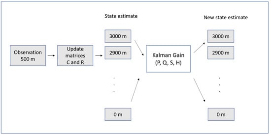
Figure 1. Diagram block describing the usage of the Kalman filter in AWEA (adapted from de Jong et al., 2014 ^[11]).

The model was tested near the Schipol airport (the Netherlands) using radar data provided by the Royal Netherlands Meteorological Institute. Two case studies were considered: the first one was an offline simulation, and the second was a fast-time simulation study into aircraft spacing. In the first case, a logarithmic wind profile calculated with a measure from an aircraft (from 0 to 3000 m) with the superposition of a normal distributed noise was used as input for AWEA. The authors used a bootstrap sample extracted from the simulation to calculate the mean and 95% confidence interval of the RMSE (Root Mean Square Error), using ten noise realizations. The numerical simulations revealed that the algorithm is able to reduce the measurement noise from 1.94 knots to 1.35 knots. Moreover, the estimated wind profile can be used to forecast the wind in locations that are positioned farther along the trajectory. The effects of the observation distance were investigated by varying the value of the parameter K_w from 0.1 to 1 in steps of 0.1. The analysis showed that the RMSE value is reduced when K_w is increased, from about 3.5 knots for K_w = 0.1 to 2.2 knots for K_w = 1, confirming the importance of distance information.

In the second case, the ground-based AWEA used broadcast measurements from the aircraft within a TMA to define a single wind profile able to represent the wind field of the entire TMA.

3. Wind Field Reconstruction with Random Fourier Features

In a recent work, Kiessling et al. ^[12] analyzed a method for wind field reconstruction based on a machine learning approach and compared it with well-established interpolation techniques. Their approach was mainly devoted to the support of wind farm planning, for which measurements are used to estimate the expected aggregate energy output. The model considered approximates data using a Fourier series, exploring the frequency domain by using a Metropolis ^[13] adaptive algorithm: at each step, the Fourier coefficients are optimized with respect to a loss function. This method does not consider previous or future time steps, then only a subset of the physical hypothesis on the system is actually applied. The model includes the hypothesis of divergence-free flux, which is always applied in the mesoscale atmospherical models ^[14]:

\nabla \cdot \vec{u} = 0

where

\vec{u}

is the velocity vector (m/s). The basic idea of random Fourier features is to define an explicit feature map that is of a dimension lower than the number of observations, but with the resulting inner product which approximates the desired kernel function. The definition of interpolation models was restricted to approximations of specific functions in a two-dimensional range, since only the horizontal wind vector is considered. Specifically, the authors defined a spatial interpolation model as a map f from a set of measurements of velocity to a vector field f_d. This process for the definition of a model f is defined as “training” and is performed by minimizing a loss function. There is an important distinction between f and f_d, since the function f represents a model that is trained on the original data and produces a vector field f_d that approximates the velocity vector

\vec{u}

. In the classical Fourier series models, the coefficients are defined as:

β (x) = {\sum_{k = 1}^{K} \hat{β_{k}} e^{i ω_{k} x}}

and the parameters

\hat{β_{k}}

are estimated by optimizing with respect to the expectation of a loss function. In the random Fourier features instead, the optimization is made with respect to the Fourier frequencies ω_k. In this view, the random Fourier features are an example of a neural network with a hidden layer and a trigonometric activation function ^[13]. In particular, ω are the weights connecting the inputs x to the hidden layer, and β are the weights connecting the nodes in the hidden layer to the output layer. In other words, it is the training algorithms that distinguish the random Fourier features.

In order to perform benchmark activities, the following classic algorithms were considered as references: nearest neighbors, inverse distance weighting (IDW), kriging ^[15], random forest, and neural network. The quality of the reconstruction with the model considered with respect to the classical models was measured using the Q(f) indicator, defined as the mean square deviation of the data provided by the model f(x) against observational data u.

Q (f) = \sum_{1}^{M} {‖f_{k} (x) - u‖}^{2}

The indicator ε(f), obtained by normalizing Q(f) with respect to the expected squared velocity, was used too. The analysis of the results showed that the random model Fourier features provide the best results against the other models tested.

4. The Meteo Particle Model (MPM)

This model was introduced by Sun et al. ^[16] with the aim of providing an estimate of atmospherical variables inside the airspace using a Monte Carlo approach, using only surveillance data from aircraft. The original method is applicable to both wind and temperature fields. The main idea is based on the usage of a stochastic process to obtain meteorological information in a short time range (from minutes to one hour) in areas where observations are lacking, starting from data collected along high-density flight trajectories. Wind and temperature states are reconstructed using virtual particles that are generated every time new observations are available (of wind and/or temperature) and that then propagate and decay over time. In this way, particle propagation allows the evaluation of atmospherical variables in those areas where measurements are not available. On the basis of the MPM model, it is possible to build a short-term wind predictor based on a time-dependent statistical model (Gaussian Process Regression, GPR). The GPR predictor can be built for each position of interest, in order to provide short-term forecasts. However, it is necessary to record a short chronology of the states estimated by the MPM model.

4.1. Selection of Input Data

The ensemble of measurements performed by the different aircraft represents a measurement array [x, y, z, u, v, T] including spatial coordinates, wind components and temperature. Initially, a probabilistic selection process is used to remove wrong measurements that could occur, specifically:

A Gaussian probabilistic function is built starting from the current field, once that mean μ e variance σ has been calculated:

p = \exp [- \frac{1}{2} \frac{{(x - μ)}^{2}}{k_{1} σ}]

In which k₁ is a control parameter defined as the acceptance probability factor.

New data selection: each new data has a p probability of being accepted, in such a way that data related to extreme values have a low probability of being selected. The numerical value assigned to k₁ is defined by the user in an empirical way, and its value can be augmented to allow a larger tolerance (increase in the number of accepted measurements). The value proposed by the authors of the method is 3.

4.2. Construction of Particles

A particle is defined as an object able to provide information on the state of wind and temperature. Particles are generated every time new wind measurements (u, v) are available: in particular, for each measurement, N particles are generated close to the position of the aircraft that performed the evaluation. Each particle is characterized by the age (set equal to zero at the time of initialization and increased at the successive steps) in such a way that, at a fixed age, the oldest particles are removed. A small variance is then assigned at the state carried by each particle, to consider the measurement uncertainties. Successively, it is assumed that particles move according to a Gaussian random walk model, i.e., the coordinates x_p, y_p, z_p (m) of the N particles (x_p,i, y_p,i, z_p,i, with i = 1, … N) at the new time step t + Δt are evaluated on the basis of the positions at the previous step t using the following expressions:

x_{p, i, t + ∆ t} = x_{p, i, t} + ∆ P_{x, i, t} y_{p, i, t + ∆ t} = y_{p, i, t} + ∆ P_{y, i, t} z_{p, i, t + ∆ t} = z_{p, i, t} + ∆ P_{z, i, t}

In which the ΔP factor is calculated as

{∆ P}_{x, i, t} = k_{2} {σ u}_{i} ∆ t {∆ P}_{y, i, t} = k_{2} {σ v}_{i} ∆ t

Along the horizontal direction (x and y), particles move according to a random track characterized by a small bias (σ), conveniently controlled by the k₂ factor (particle random walk factor). Along the vertical direction (z), the propagation follows a zero-average Gaussian track. All the particles are re-sampled at the end of each step. The time step Δt is chosen according to criteria of numerical stability, considering the time frame of the specific application, e.g., the size of the geographical domain, the time interval between two successive measurements, and the time step of the NWP (if the MPM is coupled with an NWP). The particles that for their motion fall outside the domain (both in horizontal and vertical directions) are removed, while the remaining ones are classified according to their age, according to the following probability function:

p (α) = \exp [- \frac{{(α)}^{2}}{2 σ_{α}^{2}}]

where α is a number that represents the age of the particle and σ_α is a control parameter (aging parameter). This resampling ensures a periodic particle renewal, in such a way that the oldest ones are removed.

4.3. Evaluation of Variables Value in a Generic Point

Numerical values of wind and temperature at each position can be calculated by using information carried by the surrounding particles. In particular, the wind in a generical position is evaluated as a weighted average of the wind values carried by the particles belonging to an ensemble P, which includes all the particles whose coordinates x,y,z are within a maximum predetermined distance from the coordinates of the position being considered.

u (x, y, z) = \sum_{i} W_{p, i} u_{p, i}

v (x, y, z) = \sum_{i} W_{p, i} v_{p, i}

w (x, y, z) = \sum_{i} W_{p, i} w_{p, i}

where the previous sums extended to all the particles of the P ensemble. The weight W_p assigned to each particle is calculated as a product of two exponential functions:

W_{p} = f_{d} (d) \cdot f_{0} (d_{0})

The first function establishes a relationship between the weight itself and the distance d (m) between the particle and the position considered, and the second one establishes a relation between the weight and the distance d₀ of the particle from its origin:

f_{d} (d) = \exp [- \frac{{(d)}^{2}}{2 C_{d}^{2}}]

f_{0} (d_{0}) = \exp [- \frac{{(d_{0})}^{2}}{2 C_{d}^{2}}]

in which C_d is a control parameter (weighting parameter). These formulae are based on the IDV technique (Inverse Distance Weighted) ^[17].

5. NWP Models

Limitations in the applications of wind field reconstruction methods are related to the fact that estimations can be produced only if a sufficient number of drones is already flying in the area considered; this limitation could be mitigated using measurements from ground anemometers or using data provided by Numerical Weather Prediction models (NWPs). Scientific and technological developments have led to increasing the weather forecast capabilities over the past 40 years. In ref. ^[18], Mazzarella et al. investigated if NWP-based short-range high-resolution weather forecasts (including data assimilation) can improve the predictive capability of extreme events, to understand if such forecasts can be suitable to support air traffic management. NWPs take current weather observations as input through process-defined data assimilation aimed to produce initial conditions for the meteorological variables (from the oceans to the top of the atmosphere). The derivation of the current state (the analysis) of the atmosphere is treated as a Bayesian inversion problem using observations (even from drones), previous information from forecasts and related uncertainties as constraints. These calculations involve a global minimization and are performed in four dimensions to produce an analysis that is physically consistent in space and time and can deal with observational data that are heterogeneously distributed in space and time, such as those provided by drones themselves. NWPs deliver weather forecasts by solving the full set of prognostic equations upon which the evolution in the atmosphere of wind, pressure, density and temperature is described ^[19]. These equations are solved numerically using temporal and spatial discretization, and this technique provides a distinction between resolved and unresolved scales of motion. Physical processes on unresolved scales need to be parameterized in terms of their interaction with the resolved scales. NWPs are classified into two categories: General Circulation Models (GCMs) and Limited Area Models (LAMs). GCMs perform simulations considering the global atmosphere and are characterized by a low resolution. Limited Area Models are used to obtain detailed information over a specific area of interest and they allow the usage of a higher resolution. GCMs are important also because they provide initial and boundary conditions to LAMs; in the present study, the attention is focused only on LAMs because they are widely used to support civil aviation.

6. Conclusions

The treatment of the retrieved wind field is still incomplete and a big effort from the scientific community is needed to cope with the chaotic nature of wind, the movement of aircraft, and the non-uniform distributed network of observations. In the framework of the EDUS project, CIRA is defining an operating platform demonstrator based on the existing CIRA Meteo Service Center in order to integrate data and algorithms with newer ones, aimed at treating the urban wind, in particular the evaluation of the three components from soil up to 3 km of altitudes. A promising approach could be based on the integration of monitoring “low cost and mobile” data and other sources, such as those available from the COPERNICUS program (copernicus.eu), especially for what concerns urban areas. Given the current lack of meteorological data available in urban environments, the usage of existing measurement networks will be increased, such as those coming from universities, regional agencies, civil protection and small airports. Of course, the installation of new sensors will be required, according to local stakeholders. These stations will represent the “ground truth” of remote sensing data and, along with all the data sources available, will allow the monitoring and nowcasting at high resolution of wind and other variables.

References

Barrado, C.; Boyero, M.; Brucculeri, L.; Ferrara, G.; Hately, A.; Hullah, P.; Martin-Marrero, D.; Pastor, E.; Rushton, A.P.; Volkert, A. U-Space Concept of Operations: A Key Enabler for Opening Airspace to Emerging Low-Altitude Operations. Aerospace 2020, 7, 24.
SESAR Joint Undertaking. European ATM Master Plan: Roadmap for the Safe Integration of Drones into all Classes of Airspace. Tech. Rep. Mar. 2017. Available online: https://www.sesarju.eu/node/2993 (accessed on 6 October 2023).
Fang, Z.; Zhao, Z.; Du, L.; Zhang, J.; Pang, C.; Geng, D. A new portable micro weather station. In Proceedings of the 2010 5th IEEE International Conference on Nano/Micro Engineered and Molecular Systems, Xiamen, China, 20–23 January 2010; pp. 379–382.
Rillo, V.; Zollo, A.L.; Mercogliano, P. MATISSE: An ArcGIS tool for monitoring and nowcasting meteorological hazards. Adv. Sci. Res. 2015, 12, 163–169.
Steppeler, J.; Doms, G.; Bitzer, H.W.; Gassmann, A.; Damrath, U.; Gregoric, G. Meso-gamma scale forecasts using the nonhydrostatic model LM. Meteorol. Atmos. Phys. 2003, 82, 75–96.
Zängl, G.; Reinert, D.; Rípodas, P.; Baldauf, M. The ICON (ICOsahedral Non-hydrostatic) modelling framework of DWD and MPI-M: Description of the non-hydrostatic dynamical core. Q. J. R. Meteorol. Soc. 2015, 141, 563–579.
Mondoloni, S. A Multiple-Scale Model of Wind-Prediction Uncertainty and Application to Trajectory Prediction. In Proceedings of the 6th AIAA Aviation Technology, Integration and Operations Conference (ATIO), Wichita, KS, USA, 25–27 September 2006; pp. 1–6.
Kalman, R.E. A New Approach to Linear Filtering and Prediction Problems, Transaction of the ASME. J. Basic Eng. 1960, 82, 35–45.
in’t Veld, A.C.; de Jong, P.M.A.; van Paassen, M.M.; Mulder, M. Real-time Wind Profile Estimation using Airborne Sensors. In Proceedings of the AIAA Guidance, Navigation, and Control Conference, Portland, OR, USA, 8–11 August 2011.
Zoumakis, N.M.; Kelessis, A.G. Methodology for Bulk Approximation of the Wind Profile Power-Law Exponent under Stable Stratification. Bound. Layer Meteorol. 1990, 55, 199–203.
De Jong, P.M.A.; Van der Laan, J.J.; In‘t Veld, A.C.; Van Paassen, M.M.; Mulder, M. Wind-Profile Estimation Using Airborne Sensors. J. Aircr. 2014, 51, 1852–1863.
Kiessling, J.; Ström, E.; Tempone, R. Wind field reconstruction with adaptive random Fourier features. Proc. R. Soc. A 2021, 477, 20210236.
Kammonen, A.; Kiessling, J.; Plecháč, P.; Sandberg, M.; Szepessy, A. Adaptive random Fourier features with metropolis sampling. Found. Data Sci. 2020, 2, 309.
Pielke, R. Mesoscale atmospheric modeling. In Encyclopedia of Physical Science and Technology, 3rd ed.; Meyers, R.A., Ed.; Academic Press: New York, NY, USA, 2003; pp. 383–389.
Dalmau, R.; Pérez-Batlle, M.; Prats, X. Estimation and prediction of weather variables from surveillance data using spatio-temporal Kriging. In Proceedings of the 2017 IEEE/AIAA 36th Digital Avionics Systems Conference (DASC), St. Petersburg, FL, USA, 17–21 September 2017; IEEE: Piscataway, NJ, USA, 2007; pp. 1–8.
Sun, J.; Vû, H.; Ellerbroek, J.; Hoekstra, J.M. Weather field reconstruction using aircraft surveillance data and a novel meteo-particle model. PLoS ONE 2018, 13, e0205029.
Zhou, J.; Wu, Y.; Yan, G. General formula for estimation of monthly average daily global solar radiation in China. Energy Convers. Manag. 2005, 46, 257–268.
Mazzarella, V.; Milelli, M.; Lagasio, M.; Federico, S.; Torcasio, R.C.; Biondi, R.; Realini, E.; Llasat, M.C.; Rigo, T.; Esbrí, L.; et al. Is an NWP-Based Nowcasting System Suitable for Aviation Operations? Remote. Sens. 2022, 14, 4440.
Bauer, P.; Thorpe, A.; Brunet, G. The quiet revolution of numerical weather prediction. Nature 2015, 525, 47–55.

© Text is available under the terms and conditions of the Creative Commons Attribution (CC BY) license; additional terms may apply. By using this site, you agree to the Terms and Conditions and Privacy Policy.

Upload a video for this entry

Information

Subjects: Meteorology & Atmospheric Sciences

Contributor MDPI registered users' name will be linked to their SciProfiles pages. To register with us, please refer to https://encyclopedia.pub/register :

Edoardo Bucchignani

View Times: 88

Update Date: 23 Nov 2023

Table of Contents

Video Upload Options

Confirm