Your browser does not fully support modern features. Please upgrade for a smoother experience.
Submitted Successfully!
 +1 credit
Thank you for your contribution! You can also upload a video entry or images related to this topic.
For video creation, please contact our Academic Video Service.
| Version | Summary | Created by | Modification | Content Size | Created at | Operation |
|---|---|---|---|---|---|---|
| 1 | Giordana Bonavolontà | -- | 7773 | 2023-11-04 09:06:34 | | | |
| 2 | Camila Xu | Meta information modification | 7773 | 2023-11-06 02:47:09 | | | | |
| 3 | Camila Xu | Meta information modification | 7773 | 2023-11-08 07:53:11 | | |
Video Upload Options
We provide professional Academic Video Service to translate complex research into visually appealing presentations. Would you like to try it?
Cite
If you have any further questions, please contact Encyclopedia Editorial Office.
Bonavolontà, G.; Lawson, C.; Riaz, A. Sonic Boom Prediction and Minimization. Encyclopedia. Available online: https://encyclopedia.pub/entry/51153 (accessed on 27 July 2026).
Bonavolontà G, Lawson C, Riaz A. Sonic Boom Prediction and Minimization. Encyclopedia. Available at: https://encyclopedia.pub/entry/51153. Accessed July 27, 2026.
Bonavolontà, Giordana, Craig Lawson, Atif Riaz. "Sonic Boom Prediction and Minimization" Encyclopedia, https://encyclopedia.pub/entry/51153 (accessed July 27, 2026).
Bonavolontà, G., Lawson, C., & Riaz, A. (2023, November 04). Sonic Boom Prediction and Minimization. In Encyclopedia. https://encyclopedia.pub/entry/51153
Bonavolontà, Giordana, et al. "Sonic Boom Prediction and Minimization." Encyclopedia. Web. 04 November, 2023.
Copy Citation
NASA describes the sonic boom as “thunder-like noise a person on the ground hears when an aircraft […] flies overhead faster than the speed of sound”. Sonic boom results from the coalescence of the shock waves generated by an aircraft flying supersonicly trough their propagation into the atmosphere to the ground.
supersonic aircraft design
sonic boom modeling and prediction
1. Introduction
Since the Wrights brothers’ first flight took place in 1903, flying faster has been a human dream, and as research and technology developed, especially with the introduction of jet engines, this dream started to come true. In October 1947, General Charles ‘Chuck’ Yeager piloted the Bell X-1 [1] to a speed of Mach 1.07, breaking the barrier of sound for the first time and ushering in the era of manned supersonic flight. During the years after this important event, a multitude of supersonic aircraft were manufactured exclusively for military purposes. However, in 1968, the world’s first commercial supersonic transport aircraft, the Soviet Tupolev Tu-144, took its first flight, just two months before the inaugural flight of the British–French Concorde. Tupolev Tu-144 was in passenger service in 1977 and 1978 but only on one route, completing just 55 flights. It was a commercial failure with numerous technical faults leading to reliability and safety concerns, culminating in a test flight crash in May 1978. It continued to fly until 1999 as a test vehicle. Concorde was operated from 1976 to 2003, and since that date, no other supersonic transport aircraft has flown. The main reasons for Concorde’s limited commercial success were the high fuel consumption linked to the high thrust needed, high operational costs and the impact of the sonic boom produced on the environment and communities. In 1978, an FAA regulation restricted the operation of civil aircraft at speeds greater than Mach 1 overland. This severely limited the routes viable for Concorde and discouraged the interest in developing new supersonic civil aircraft for a long period of time. This fact if, on one hand, blocked the market for supersonic aircraft, on the other hand raised great interest in the sonic boom phenomenon, and considerable investigation and research, aiming at understanding the phenomenon and predicting it, were undertaken over the following decades. NASA describes the sonic boom as “thunder-like noise a person on the ground hears when an aircraft […] flies overhead faster than the speed of sound” [2]. Sonic boom results from the coalescence of the shock waves generated by an aircraft flying supersonicly trough their propagation into the atmosphere to the ground. Here, a strong and impulsive pressure change is generated that may damage structures and annoy, in a not acceptable way, people. According to Coulouvrat [3], it seems that the sonic booms generating at cruise altitudes are not harmful in terms of intensity, but high adverse reactions might be expected from people likely to be frequently exposed to even low-level booms. It can have a negative impact also on marine and wildlife [4]. The typical sonic boom signature at the ground is the so-called “N-wave” (Figure 1), which is characterized by sharp pressure jumps at the front and back of the waveform, with a slow pressure drop in between. Sonic boom intensity and its extension on the ground depend mainly on aircraft weight, size, altitude and Mach number. The area affected by a sonic boom is called the ‘boom carpet’ and can extend up to 70 miles behind the aircraft [5].
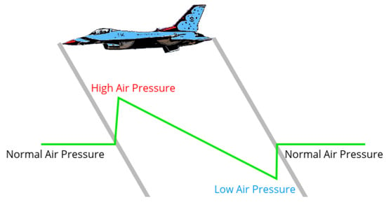
Figure 1. Typical N-wave sonic boom signature at ground (source: [6]).
Several factors, such as variation in signature shape, pressure levels, rise time and frequency content, seem to have a large influence on the resultant sonic booms disturbance level [7]. These are, in turn, affected by environmental conditions, making sonic boom a real complex phenomenon to be analyzed and modeled. In the last 20 years, the encouraging results of the previous studies and research, along with the developments in the aviation industry and the introduction of increasingly advanced technologies, have led many companies to strongly invest in the design and development of the new generation of supersonic aircraft. At the same time, the ICAO (International Civil Aviation Organization) Committee on Aviation Environmental Protection is working to develop new certification standards for supersonic aircraft and environmental regulations in terms of sonic boom, noise and emissions [8]. The FAA is gathering data and information from sonic boom flight test campaigns to determine whether to amend the current ban on supersonic flight by civil aircraft overland in the United States [9]. Sonic boom reduction and mitigation constitutes supersonic flight’s biggest challenge. However, the reintroduction of supersonic aircraft needs also to address high efficiency and low climate impact, and must be economically and commercially viable. Although some conventional aircraft designs have proven that they can be carefully shaped and optimized in order to obtain lower levels of both sonic boom and wave drag, it seems to be insufficient to attain sufficient noise reduction. In addition, other stringent requirements on LTO noise, high-altitude NOx emissions and fuel consumption would be difficult to meet. A technological breakthrough is needed for the design of a new generation of supersonic transport aircraft. In order to achieve this, it seems necessary to explore a multitude of different and unconventional aircraft configurations, together with careful airframe–engine integrated design. Provisions should be made, as necessary, for appropriate noise reduction systems and measures, and the evaluation of their impact at the aircraft level is of vital importance. A multi-disciplinary optimization (MDO) approach is needed, and sonic boom prediction and minimization must be in the loop within the very first steps of the process.
2. Sonic Boom Prediction and Minimization
NASA describes sonic boom as a “thunder-like noise a person on the ground hears when an aircraft […] flies overhead faster than the speed of sound” [2]. Sonic boom results from the coalescence at the ground of strong, impulsive shock waves generated by aircraft flying at supersonic speed. The noise generated on the ground may damage structures and disturb people. Additionally, it can have a negative impact on marine and wildlife [4]. Sonic boom intensity and extension on the ground depends mainly on aircraft weight, size, altitude and Mach number. The area affected by a sonic boom is called the ‘boom carpet’ and can extend up to 70 miles behind the aircraft [5]. Sonic boom mitigation remains supersonic flight’s biggest challenge, and a large number of studies and research projects have been carried out since the 1950s in order to understand the phenomenon and accurately model it. Sonic boom prediction is, in fact, a requirement for both advanced supersonic transport design, and environmental assessment tools of various military and aerospace activities. The problem of sonic boom modeling and prediction can be divided into two main parts: prediction of the near-field pressure signature and its propagation to the ground. The physical domain can be divided into three parts, as shown in Figure 2, according to the pressure signature evolution occurring during its propagation through the atmosphere. Generally, the near-field is considered to be a region small enough that atmospheric gradients do not play a significant role. This is usually a few body lengths. Mid-field is where significant nonlinear distortion of the signature has occurred, but geometric features of the aircraft are still apparent. The far field is where the signature approaches an asymptotic shape [10]. The far-field condition is not always reached at ground: for large aircraft, cruising at high altitudes, in fact, ground signatures can still be mid-field.
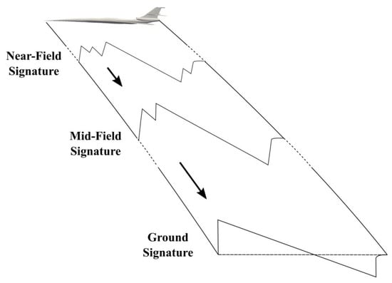
Figure 2. Sonic boom generation, propagation and evolution. Source: [11]).
2.1. Prediction Methods
2.1.1. Fundamental Theory
The fundamental theory for sonic boom modeling and prediction was established in the 1950s with Whitham’s works [12][13]. He developed a modified linear theory for the prediction of the sonic boom generated by an axisymmetric non-lifting slender body in a straight supersonic flight at a constant Mach number. The method is based on linearized supersonic flow theory [14] and the supersonic area rule [15][16] for near-field pressure signature calculation, and the geometrical acoustics method [17] for acoustic propagation. It also accounts for shocks and other nonlinear characteristics existing in real flow and which accumulate as far as one moves away from the body [18] by means of nonlinear steepening and application of the so-called Whitham rule. The effect of wind, density and temperature gradients as well as aircraft maneuvers are included.
Whitham’s theory can be summarized in three steps:
-
The acoustic source signature of the vehicle is obtained in terms of a normalized form known as the Whitham F-function. It represents the axisymmetric (or locally axisymmetric) linear acoustic solution in a uniform medium.
-
The F-function is extrapolated to large distances by using geometrical acoustics ray tracing, requiring as inputs the vehicle trajectory and the structure of the atmosphere, and according to which the amplitude changes but the shape is fixed.
-
In the end, Whitham’s rule is applied to the complete linear acoustic signature. This accounts for nonlinear steepening or “aging” of the signature. Shocks fitting is carried out such that the total area is conserved (‘area balancing’ rule).
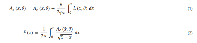
In 1955, Lomax [19] generalized the modified linear theory for arbitrary lifting configurations, showing that the axisymmetric body area rule can be generalized to asymmetric bodies, including the effects of lift, and Walkden, in 1958, applied these findings to sonic boom prediction [20]. The cross-sectional area distribution 𝐴(𝑥) in the F-function (Equation (2)) was substituted by an equivalent area 𝐴𝑒(𝑥,𝜃) distribution (which is a function of the azimuthal angle, or angle in the roll direction) comprising both volume and lift contribution (Equation (1)):
In the years following, several studies [21][22][23] validated the fundamental theory, and by the early 1960s, it was well established. It included arbitrary aircraft maneuvers, ray tracing through a horizontally stratified atmosphere with winds, and evolution of the far-field boom for an arbitrary F-function. The first and successful implementation of sonic boom fundamental theory was the Hayes, Haefeli, and Kulsrud code in 1969, known as the Hayes program or ARAP (Aeronautical Research Association of Princeton) program [24]. The program requires as input an F-function source and implements a ray-tracing formulation analytically derived from Fermat’s principle. Whitham’s rule is applied via the concept of signature aging, and shock coalescence is handled by numeric area balancing. ARAP made a major breakthrough in sonic boom research since it was the first code to apply the well-developed theory of geometrical optics to an acoustic problem. In 1972, Thomas [25] published a code that used a quite different algorithm for signature propagation. Thomas’ program computes ray paths by direct numeric integration of the eikonal (by applying Huygen’s principle) and applies Whitham’s rule via the analytic waveform parameter method. A set of parameters is defined for a waveform complete description, and equations are obtained for the time rates of change of these parameters. Rather than beginning with an F-function, Thomas’ program input is Δ𝑝 longitudinal distribution at some radius. Whitham’s and Thomas’ methods are mathematically equivalent and give the same results since both represent the full implementation of fundamental theory, but the waveform parameter method appears to provide a more suitable approach for automatic computation [25][26]. In addition, Thomas’ program provides the user with the possibility to directly input the pressure signature around the body from wind tunnel tests or CFD, instead of calculating it from the F-function. In fact, even if these two quantities are directly related, the actual Δ𝑝 in the near-field does not necessarily correspond to the effective Δ𝑝 from the F-function. This becomes significant especially when complex, low-boom-shaped configurations are analyzed. Both Hayes’ and Thomas’ programs are essentially single-point programs: one run of either yields the boom at a single azimuth and flight time. This can cause stacked runs to be applied if a full mission analysis is required. These two programs are still actively used today, and represent a reference for what are termed full ray trace programs. Virtually every full ray trace sonic boom program is evolved in one way or another from one of them. One example is the first version of NASA PCBoom [27][28], which is an extension of Thomas code. Simplified implementations of fundamental theory are given instead in [29][30]: these are valid for analyses in a windless atmosphere. The first work by George and Plotkin [29] presented charts that allow the manual computation of signature evolution under the flight track. Carlson [30], on the other hand, developed a very useful handbook procedure for a “first-cut” estimation of far-field booms generated by steady flight in a standard atmosphere, where the ground signature is expected to be an N-wave. He provided equations similar to Whitham’s far-field formulas but with several factors associated with propagation. These factors include the effect on amplitude and duration due to refracted ray paths and acoustic impedance gradients, and amplification due to reflection at the ground. Propagation off-track is included. The integral of the F-function is represented by a normalized shape factor scaled according to aircraft size [10]. Shape factors for several airplanes are given in a chart, and a simple procedure allows the calculation of it for types of aircraft not included in the chart. Refraction and impedance factors for flight in a standard atmosphere are contained in charts as well. With Carlson’s method, an estimate of both overpressure and N-wave duration can be obtained. Carlson’s method is valuable not only because it allows quick calculations of steady flight N-wave booms but also because it explicitly shows the scaling effect of parameters such as Mach number and aircraft length. Additionally, the shape factors can be used to generate effective F-functions to be used in full ray trace programs. This method is validated against numerical simulations (full CFD approach) in [31]. The agreement between the two methods occurs in the limits of validity of the N-wave model. Nevertheless, the Carlson method can be easily applied during the preliminary design of a supersonic aircraft with the purpose of selecting the baseline geometry on which to perform the optimization process through the CFD computations. A new empirical formulation to obtain useful predictions of the magnitude and footprint of the sonic boom that would be created by either known supersonic aircraft or new designs flying at a constant Mach number and altitude was developed in 2006 by Clare [32]. This research is based on the linear regression of independent parameter groups operating on the Lee and Downing 1991 database [33] of sonic booms created by military aircraft at Edwards Air Force Base, California, USA. The formulation employs an empirical F function that characterizes the near-field effects of shape, lift, and Mach number on the sonic boom. The prediction accuracy, as assessed by the scatter within the original database, is retained acceptably, and able to produce better correlations with respect to alternative analytical prediction models. However, the formulation can only make predictions of sonic booms generated by flying at a constant altitude and Mach number, and cannot make predictions for maneuvering aircraft. Summarizing, fundamental theory can provide accurate predictions of the sonic boom ground signature produced by supersonic aircraft, but some limitations arise from the assumptions on which it is founded.
Being the fundamental theory founded on linearized supersonic flow theory, it is valid just for slender bodies at moderate supersonic Mach numbers in inviscid and irrotational flow. Above Mach 3, in fact, slender-body theory does not provide reliable results [5]. Standard theory represents shock waves in the traditional gasdynamic form of zero-thickness pressure jumps. Real sonic boom shock waves have a finite rise time, occurring partly from turbulence and partly from molecular relaxation, which affects the high-frequency content of the boom spectrum. These frequencies are important for some human response loudness assessment techniques [34], and, for this reason, an artificial shock thickening method is required. Additionally, assumption of the N-wave signal at ground independently from the aircraft shape is made by Whitham [12]. In 1965, McLean showed for the first time that for a representative supersonic aircraft, the signature would not actually reach the asymptotic state at ground until much further than a cruise altitude of 44,000 feet [35], and the distances at which far-field is reached depend on the shape of the aircraft. Furthermore, in real atmospheric conditions, characteristics coalesce more slowly than in uniform atmosphere, increasing the possibility that non-fully coalesced N-wave signatures shapes may reach the ground. In the end, turbulence, as well as atmosphere variability and absorption effects, are not accounted for in pressure signature propagation. In particular, turbulence modeling, although difficult, results to be of particular interest as to whether the waveform distortion caused by its presence will adversely affect the loudness of minimized sonic boom signatures associated with low-boom supersonic transport. The fundamentals of sonic boom theory were established and validated in the 1950s and early 1960s, and since then, there has been significant research and advances in both the understanding and modeling of sonic boom. The substantial growth in computing power and its widespread availability have allowed for the development and use of more sophisticated prediction methods and tools. These include full CFD solutions for the near-field pressure signature computation, and the iterative resolution of the augmented Burgers’ equations for signature propagation to the ground. Turbulence and nonstandard atmosphere effects could even be modeled and included.
2.1.2. Advances in Near-Field Prediction
Near-field pressure signature prediction according to Whitham’s theory provides that the effect of geometry and lift must be modeled with an equivalent axisymmetric body of revolution, and as the complexity of the geometry increases, this process becomes difficult [36]. A solution to that is given by using Euler CFD solutions to obtain the near-field pressure signature [37][38][39][40]. CFD makes it possible to treat a model of real aircraft geometry without any simplification or transformation. Moreover, by running viscous as opposed to inviscid simulations, more accurate pressure information can be extracted, and plume effects [41], as well as inlet integration [42] can be taken into account. The complexities associated with such a numerical method mainly relate to the fact that a careful grid generation is needed to properly define the computational domain, and solutions become increasingly more expensive as the domain size increases. An obvious approach to using CFD would be to extend the domain and carry the calculations out to distances, where a far-field condition is met. However, for complex configurations, such as low-boom supersonic transports, this condition may not be met, even at distances of five or ten body lengths [38]. The cost, in terms of both computational power and time, is high, especially when the domain must be extended out far enough so as to correctly match the three-dimensional CFD solution with the one-dimensional propagation models (or to convert CFD pressure signals into equivalent far-field radiating source distributions [10]). Although some techniques have been developed to match the three-dimensional near-field solution provided by CFD with the propagation codes [37][43][44][45], by allowing for a smaller domain to be used for the near-field solution, as computational technology has continued to grow rapidly and solutions methods have improved, it has become common to increase the domain size enough to provide a pressure signature that is well approximated as one dimensional. This still comes at a high computational cost. As a result, CFD solutions are not suitable for applications such as trade-off studies or optimizations that involve a big number of configurations to analyze, typically carried out during conceptual and preliminary aircraft design stages. On the other hand, high-fidelity methods are the only available solution for detailed design and/or multi-disciplinary optimization studies. A reasonable trade-off consists in implementing CFD solutions to build response surfaces or surrogate models. Another option to obtain the near-field pressure signature around almost any complex geometry with a computational cost that is orders of magnitude smaller than a full CFD solution is to use 3D high-order panel methods [46][47][48]. These methods, developed heavily in the 1970s and 1980s, can provide a linearized inviscid supersonic solution of the near-field flow around the aircraft and have been used in optimization studies of low-boom configurations [49][50][51]. Even with panel methods, the geometry is modeled directly. Consequently, three-dimensional effects, such as lift and shielding effects, are determined without the need of generating equivalent axisymmetric bodies as in classical theory. However, since they provide a linearized inviscid solution, their use is restricted to slender bodies at low Mach numbers. Unlike full CFD, panel methods can provide a near-field solution at any distance away from the aircraft without additional computational costs. However, since this solution is linear and assuming a uniform flow field, the error increases with distance. Chan [49] proposed a methodology for correcting the error due to the linearity of the panel solution. It involves calculating the near-field signature by using a panel method, finding an equivalent axisymmetric source distribution, and then using the fundamental theory. This takes into account the nonlinearity, to calculate a new near-field corrected signature. According to Giblette [46], panel methods for near-field pressure signature prediction give results that are in good agreement with CFD for a simple axisymmetric geometry, while comparisons made on more complex geometries highlight the shortcoming of using a potential flow solution, in which unrealistically large velocities are calculated on sharp corners (in the case of a wing-body configuration, i.e., it could happen at the wing tip and on the side of the fuselage tail). Panel solutions show local large spikes in the signature that do not exist in the CFD signature, and that results in local large differences in both the ground signature and perceived loudness. Another solution could be the revisited version of the fundamental theory presented in [36]. Whitham’s F-function is substituted by a modified Lighthill F-function to generate the near-field pressure signature. The derivation of Lighthill’s F-function does not require the assumption of a smooth area profile as in the case of Whitham’s F-functions. This is a significant improvement, which allows Lighthill’s F-function to be applied to objects that have discontinuities. The study demonstrates that the modified Lighthill method is able to predict the sonic boom shape, magnitude, and duration within 10% with respect to pressure profiles from wind tunnel experiments, computational fluid dynamics, and flight tests, and account for variations in lift, Mach number, and propagation angle. However, in general, modified linear theory is capable of producing a first-order pressure profile, as long as the aircraft model can be resolved into an axisymmetric area profile. With run times less than a minute, and considering that no mesh generation is required, it is appropriate for the preliminary and conceptual design stages of quiet sonic boom aircraft. Summing up, the modified Lighthill function and panel methods represent a good approach for design space exploration or preliminary optimization studies of low-boom aircraft configurations, where large numbers of basic geometries are analyzed and approximate results are sufficient. These methods can also be used to generate surrogate models, even together with high-fidelity level ones [48] in a multi-fidelity framework.
2.1.3. Advances in Pressure Propagation
As in the case of near-field solutions, new methods and models have been developed even for the propagation of signatures to the ground. They try to overcome the limitations inherited with the application of fundamental theory. In particular, fundamental theory is not able to predict the shock rise time since weak shock theory assumption is made. The predicted ground signatures using traditional approaches present the shocks as discontinuous jumps, and during the calculation of the frequency spectrum and successive noise metrics, empirical or numerical shock thickening, as well as the shock-merging procedure, must be taken in place to correct or adjust the signature. This is essential because Fast Fourier Transform (FFT) and other numerical techniques required in computation of any noise or loudness metric cannot be applied to a waveform with discontinuities. However, the shock-thickening and -merging processes are subject to errors since rise times calculated are heavily dependent on the empirical or numerical factors chosen for converting the discontinuous shocks into continuous profiles, and may produce loudness or other noise metrics that are not accurate [52]. This becomes a problem especially during optimization studies, where the optimizer could exploit the shock-merging process to its advantage. Several research studies have looked at boom prediction methods that compute the rise times, instead of empirically adjusting or correcting the ground signature, resorting to weak shock theory and area balancing. The most used method is to account for molecular relaxation (a dominant mechanism in sound absorption for the frequencies typically associated with sonic booms (e.g., 1–100 Hz), responsible for thickening the shocks), absorption, atmospheric stratification and spreading terms in the governing equation, called the augmented Burgers equation [52][53][54][55]. Augmented Burgers equations differentiate from regular equations that just account for the nonlinear term. Burgers’ equation describes the evolution of the acoustic field along a ray-theoretic propagation path [56]. The classic way to solve the augmented Burger equation is by means of the operator-splitting method [50]. In 2015, Yamamoto et al. [57] proposed a different approach (“Burgers-Relax-Uni”) to solve the augmented Burger equation. An internal variable is introduced, which can be solved analytically at each step. As a result, the decomposed equations with the internal variable can be solved as a system of equations by being lumped into a matrix form. This algorithm demonstrated to be almost twice as fast as the original method and more stable. It can suppress the numerical oscillation of propagating boom at high altitude. Furthermore, different algorithms exist to handle propagation mechanisms. Some methods, like the one presented by Pilon [55] or the one developed by Robinson [54] and implemented in ZEPHYRUS code, uses the frequency domain to account for the dissipation and relaxation. Others methods, like the one from Cleveland [53], successively extended by Rallabhandi [52] in sBOOM, implements a time domain algorithm to account for all the propagation mechanisms.
Frequent conversion from the time domain to frequency domain and back during atmospheric propagation may lead to numerical errors. Even if these can be bounded, frequent FFT and inverse FFT operations add an additional computational load during the propagation process. The most relevant limitation connected with codes that solve the augmented Burgers equation is the longer computation time needed for calculating the sonic boom footprints, with respect to the ones which implement the fundamental theory. On average, the time to run such a codes is about 20–25 times slower than linear codes [52].
Another advanced propagation method is developed by solving a Full Potential Equation (FPE) to the ground [58]. This three-dimensional CFD method can march the solution with atmospheric changes in pressure and temperature taken into account. The nonlinearity and nonaxisymmetry of the Full Potential propagation code makes it superior with respect to the other prediction methods that implement the linear ray-tracing approach. However, it needs better validation against numerical and experimental measurements. Advances have also been made in the modeling and prediction of other atmospheric phenomena that could affect the sonic boom waveform at the ground, and, as a consequence, their loudness and annoyance levels. One important phenomenon having a great impact on sonic boom is turbulence. The effect of atmospheric turbulence on a sonic boom can be interpreted as a smoothing deformation of the wavefront due to both velocity and temperature turbulent fluctuations in the medium through which it propagates. In particular, there is a ragged fine structure behind each shock, and the shock rise times tend to be longer and variable [10] (Figure 3). The essence of the effect of atmospheric turbulence on sonic boom waveforms is the scattering of acoustical waves and a series of focused/defocused wavefronts.
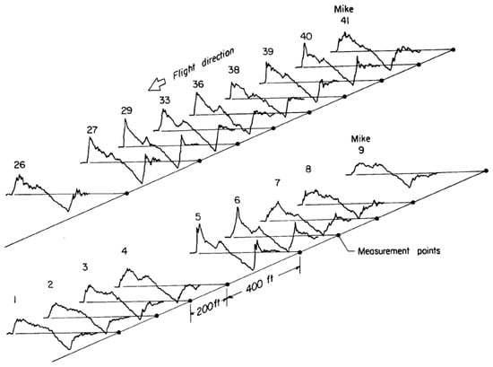
Figure 3. Sonic booms measured under calm and turbulent atmospheric conditions [59].
The effect of atmospheric turbulence on sonic booms has been investigated theoretically, experimentally, and numerically. Crow [60] first explained the fine structure by scattering theory and estimated the order of the rise time due to atmospheric turbulence from his insightful theory based on a statistical approach. Based on Crow’s estimation, Pierce [61], Pierce and Maglieri [62], and Plotkin and George [63] independently developed more detailed estimations of rise time and considered the means by which atmospheric turbulence lengthened it. Turbulence that affects sonic boom signature propagation is known as the planetary or Atmospheric Boundary Layer (ABL) because it is limited to propagation from altitudes up to 6 km. The ABL varies daily and should be modeled as both random temperature and velocity fluctuations fields. Therefore, turbulence effects are predicted by calculating sonic boom propagation through an ABL model. In order to propagate sonic boom pressure signatures accounting for turbulence distortions, the augmented Burgers equation alone is not sufficient. Useful results have been obtained by using the Khoklov–Zabolotskaya–Kuznetsov (KZK) equation as a propagation equation [59][64][65]. Turbulence model research codes based on this equation solution have been developed within the Sonic Booms in Atmospheric Turbulence (SonicBAT) Program by NASA and incorporated into the PCBoom sonic boom prediction software to estimate the effect of turbulence on the levels of shaped sonic booms associated with several low boom aircraft designs [66]. Other nonlinear models have also been applied to sonic boom propagation, including a a time domain solution of the nonlinear progressive wave equation (NPE) [67], a combined time domain and spectral approach called FLHOWARD [68] using a partially one-way equation and a similar but one-way equation called HOWARD [69][70]. The latest methodology has been implemented in a code developed in 2021 called SPnoise for Sonic Boom [71]. KZK implementation assumes what is termed the parabolic approximation, including the assumption that propagation is primarily in one direction but is better-behaved at domain boundaries than the NPE solution and the computation does not require the FFTs used in FLHOWARD or HOWARD. On the other hand, the solution of KZK may be sufficient if the solution of interest is close to the sound axis, but when the scattering is widely distributed, it results in an unsatisfied description of distorted signatures [71]. An atmospheric turbulence model is also needed in conjunction with a propagation equation to simulate a random turbulent field throughout the domain. Turbulence is represented as both temperature and wind fluctuations, usually taken from measurements or inferred. In [72], the great influence of atmospheric turbulence parameters on both classic N-waves (on which turbulence has greater influence) and low boom pressure signatures at the ground is shown, highlighting the need of stochastic studies. Another important phenomenon that needs to be carefully predicted and simulated is focused booms. Focused booms develop during supersonic aircraft accelerations in climbing, turning and maneuvering (Figure 4): although most focus booms can be avoided or minimized, the transition focus during acceleration from subsonic to supersonic speeds is unavoidable. Hence, its evaluation becomes fundamental for future low-boom aircraft in order to assess the acceptability of overland supersonic flight. Focused boom, also known as ‘sonic superboom’ leads to the amplification of ground pressures up to two or three times the carpet boom shock strength [73]. The focusing of shock waves occurs at surfaces called caustics. Caustics are surfaces where the ray tube area vanishes and geometrical acoustics becomes singular, predicting infinite overpressures. Factors which are neglected in the development of geometrical acoustics become important at focal points and serve to limit pressures to finite values. Substantial research on the behavior of a sonic boom at focus has been conducted over the past decades. The equation that describes the sonic boom pressure signature near the caustic is the nonlinear Tricomi equation, which includes diffraction effects neglected in standard sonic boom theory, as well as the usual first-order nonlinear term. Both of these limit the amplitude of the focused booms. The diffraction limit is frequency-dependent, affecting low frequencies more than high frequencies, leading to a characteristic U-wave shape with the shocks peaked (Figure 4).
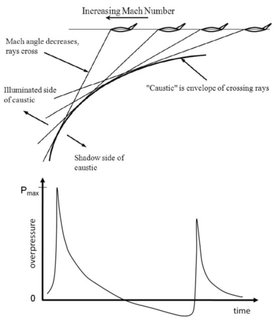
In 1965, Guiraud [76] wrote the equations for the focus of weak shock waves and developed a scaling law, while Seebass [77] found a way to linearize the Tricomi equation through a Legendre transformation. If no shock is present near the caustic, his transformation effectively linearizes the problem. Gill and Seebass [78] obtained a numerical solution for the focus of a step function at a caustic. Using Guiraud’s scaling law, Plotkin and Cantril [79] extended PCBoom to apply Gill and Seebass’ solution at focal zones. That code has evolved into PCBoom3 [10]. Marchiano and Coulouvrat [80] re-derived Guirads’ formulation of the nonlinear Tricomi equation, while Auger and Coulouvrat [81] presented an algorithm to solve the nonconservative, nonlinear Tricomi equation by using a Fast Fourier Transform. Kandil and Zheng [82][83] presented a different approach by splitting the Tricomi equations into the linear unsteady Tricomi equation and the nonlinear unsteady Burgers equation. Three computational schemes were developed: a frequency domain Fast Fourier Transform scheme, a time domain finite difference scheme and a time domain finite difference with overlapping grid (OLG) scheme. Piacsek in [84][85] instead used the nonlinear progressive wave equation (NPE) as a prediction method for focused booms. A study conducted at NASA in 2012 [86] aimed at comparing different prediction methods with flight test field measurements, showed that the Gill–Seebass method tends to overpredict local peaks, and thus, it is not applicable to complex signatures. In contrast, the NTE method with absorption appears to be better suited to the prediction of complex signatures, such as low-boom shaped signatures. Methods resulting from these studies have been implemented in sonic boom propagation codes. Aside from PCBoom3, TRAPS [87] accounts for the passage of a boom through caustics via a Hilbert transform. It is successful in predicting where focusing reaches the ground, but it gives excessively large amplitudes. ZEPHYRUS [54] tends to resolve the discrepancy of TRAPS by incorporating the air absorption effects. It predicts lower values for the overpressure as compared to TRAPS but is much more computationally intensive. In 2017, Rallabhandi [88] developed a way to numerically predict focused sonic boom signatures using both Gill–Seebass similitude and the solution to the non-linear Tricomi equation to be included in sBOOM.
2.2. Loudness and Annoyance Metrics
When an analysis of sonic boom caused by a supersonic aircraft is carried out, not only is the prediction of the phenomenon important but also the quantification of the annoyance caused to people (outdoor and indoor), the magnitude of structure vibrations and the measure of secondary effects, such as rattle. In this regard, the selection of metrics able to reflect sonic boom effects is one important step in evaluating the potential impact of introducing civil supersonic flight overland. However, still today, a unique acoustic measure to define boom acceptability levels is not established yet. Important research centers, like NASA and JAXA, have conducted several surveys, laboratory studies and low-boom flight tests to identify the correlation between metrics and sonic boom, with the aim to support and help ICAO in developing new certification standards. The European project RUMBLE (RegUlation and norM for low sonic Boom LEvels) [89] also plays a role in this regard. The project is, in fact, dedicated to the production of the scientific evidence requested by national, European and international regulation authorities to determine the acceptable level of overland sonic booms and the appropriate ways to comply with it. The main actions of the project are the development and assessment of sonic boom prediction tools, study of the human response to a sonic boom, and validation of the findings using wind tunnel experiments and actual flight tests.
Different metrics could be retained as an objective for sonic boom reduction and minimization. They can be categorized as pressure based or loudness based. To the first category belongs the maximum peak overpressure, front shock overpressure, sum of the shock amplitudes, while Sound Exposure Level (SEL), A-weighted Sound Exposure Level (A-SEL), C-weighted Sound Exposure Level (C-SEL) and Perceived Loudness deciBel (PLdB) belong to the second one. Pressure-based metrics are the most used in optimization problems, but they do not provide a cost function that synthesizes at the same time the energy content and the full frequency of the signature. Loudness metrics, instead, result from the mathematical process of the signal: it causes the loss of direct dependencies between the geometry (the input of the problem) and the metrics (the output of the mathematical system), but, on the other hand, brings the energy and frequency content of the signal that has a direct impact on the annoyance evaluation. It is clear that the choice of such an objective function is not a trivial process and results from a compromise between the accurate description of the physical phenomenon and correlation between the function itself and the design variables.
In [90], loudness and short-term annoyance ratings were collected for conventional and low-boom signatures at low overall levels. The average annoyance ratings were best reflected by ASEL (A-weighted Sound Exposure Level) values compared to other frequency weightings. Moreover, the results of the listening experiments showed that the tested low-boom designs are similarly loud and annoying as conventional and N-wave sounds when presented at similar ASEL values, and an indication of a systematic benefit for low-boom signals compared to conventional booms was not observed. However, other studies [91][92][93] indicate that psycho-acoustic loudness models or the inclusion of a loudness derivative and duration for the description of the sound character in multi-metric annoyance models can enable a better characterization of the perception of transient sounds than single level-based measures. Metrics including time-varying loudness models, such as those developed by Glasberg and Moore [94] or Zwicker and Fastl [95], may be useful for predicting the impact of impulsive sounds since they incorporate models of the temporal behavior of the human hearing system, which is clearly of importance with rapidly changing sounds. The output from their models is a profile of the loudness heard through time as opposed to a single number representing the whole or part of a sound event. Moreover, it has been noted [96] that sonic boom pressure signatures measured using microphones on the ground are different at different locations, even though nothing about the aircraft or its speed has changed. This is due to the turbulence effect, and makes it even harder to define a standard method of measurement and evaluation. An attempt to find metrics more stable to turbulence was made in [97]. According to this work, B-SEL could be a good candidate for certifying supersonic aircraft for overland civil transportation.
Another relevant topic is the difference between indoor and outdoor sonic boom effect. In 1993 [98], the sonic boom simulator of the Langley Research Center was used to quantify subjective loudness and annoyance response to simulated indoor and outdoor sonic boom signatures. Two indoor listening situations were simulated: one with the windows open and the other with the windows closed. The results were used to assess loudness and annoyance as sonic boom criterion measures and to evaluate several metrics. The findings indicated that loudness and annoyance were equivalent criterion measures for outdoor booms but not for indoor booms. Annoyance scores for indoor booms were significantly higher than indoor loudness scores. Thus, annoyance was recommended as the criterion measure of choice for general use in assessing sonic boom response. Perceived Level [99] was determined to be the best estimator of annoyance for both indoor and outdoor booms, and of loudness for outdoor booms.
The Okhlahoma city survey [100] showed that the best correlation with the annoyance is achieved using the number of boom per day. The survey recommends a boom peak pressure level of 35.91 , where N is the number of boom per day.
When it comes to the evaluation of sonic boom indoor perception, not just the audible component of the signal should be considered. Tactile motion of the building, as well as rattling (occurring for structural elements not well mounted or constrained) of the building and of the objects inside the building must be taken into account, and the last two require the introduction of a dynamic model of the structure. The simplest approximation is the lumped parameter single degree of freedom model [101] but is obviously a limitation. The wall dynamic behavior is, in fact, always coupled to the interior, and a multimodal analysis is required [102].
Figure 5 provides a summary of the main metrics suggested to be adopted as more representative of the sonic boom effect, and can be used for optimization problems, along with reference values.
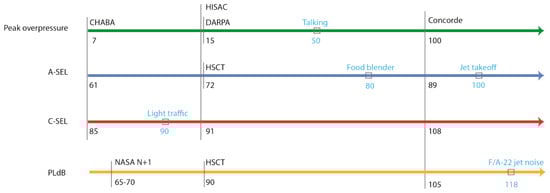
Figure 5. Sonic boom metrics proposed compared to reference values linked to ordinary events [103].
2.3. Minimization Theory and Techniques
Sonic boom minimization became of great interest during the 1960s and 1970s, when knowledge of the phenomenon’s physics and its calculation and prediction was already assessed. The first theoretical approach used as a key point was Whitham’s F-function since it constitutes the link between the aircraft configuration and the pressure signature. Jones [104] and Carlson [105] were the first to suggest that a reduction in the sonic boom could have been achieved by aircraft shaping. Based on the assumption that all pressure signatures reaching the ground would have the characteristic N-wave form, they defined an equivalent-body shape, which can produce an N-wave signature with a “lower bounded” over pressure and impulse. The area distribution they ended up with was extremely blunt, and the shape changes required to produce such equivalent areas resulted in being detrimental in terms of drag [106]. Later, in 1965, McLean found that during transonic acceleration, the signature created by large and slender SSTs might not necessarily attain their far-field N-wave form, and Hayes pointed out that in the real atmosphere, characteristics coalesce more slowly by making it possible to “freeze” the shape of the midfield signature and keep it until the ground [107]. Since the shape of a midfield signature strongly depends on the shape of the aircraft, such shaping was recognized as a much more powerful way of minimizing the boom.
George and Seebass [108][109] developed a relatively complete theory, in which they found the lower bounds for the bow and the tail shock of a midfield signature. It laid the theoretical foundation for the sonic boom minimization method. However, the nose shape determined by the minimized area distribution was as blunt as in the previous theories, with the consequence of a significant drag penalty. The low boom–high drag paradox is shown in a scheme in Figure 6. In addition, this method sacrificed the front fuselage size, resulting even in the reduction in usable fuselage space. Darden, in 1979 [110], advanced the George and Seebass’ method by controlling the bluntness of the area distribution near the nose, overcoming the drag rise problems associated with the previous theory.
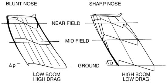
Figure 6. Low boom–high drag paradox (Source: [107]).
The final theory is known as Seebass–George–Darden, SGD, theory. It states that, given the flight conditions of altitude and Mach number and the aircraft parameters of weight and length, the equivalent area distribution needed to create either a minimum overpressure signature or a minimum shock signature can be defined. Carlson and Mack [111][112] applied the minimization method to several conceptual aircraft and ran a wind-tunnel test program to validate it. The Shaped Sonic Boom Demonstration (SSBD) program successfully tested the low-boom theory to be reliable under actual flight and atmospheric conditions.
Lately, Mack [113], Rallabhandi [114] and Plotkin [115] extended and generalized the SGD theory, by making it more flexible with respect to the trade-off between boom minimization and other performance measures, and more suitable for practical design. They also provided lower bounds for the perceived loudness.
The SGD sonic boom minimization process produces cross-sectional area profiles that generate either a minimum overpressure “flat-top” signature (Figure 7b) or a maximum-rise-time boom, which has a small initial shock pressure rise (ISPR) followed by a gradual increase to the peak overpressure (Figure 7c). These sonic boom types are essentially modified N-waves. Another option to reduce the annoyance of the sonic boom to humans is to generate a multishock signature (Figure 7d) by means of a lobe-balancing method [116][117]. Lobes are created using lift, by trimming lifting surfaces to obtain a frozen, shock balanced F-function, like the one showed in Figure 8, at different flight conditions.
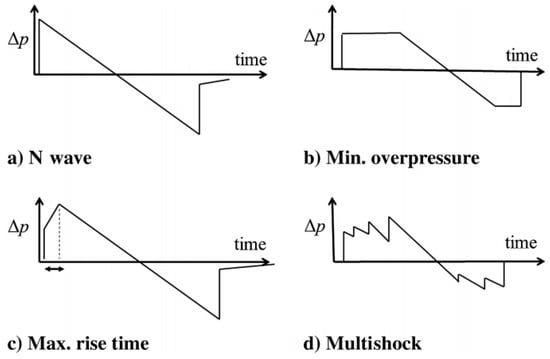
Figure 7. Types of sonic boom signatures (Reprinted/adapted with permission from Ref. [116], copyright 2023, Jung, T.).
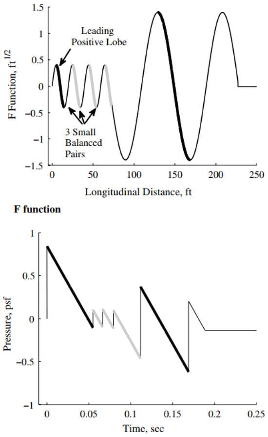
Figure 8. Example of a lobe-balanced F-function and corresponding ground pressure profile (Reprinted/adapted with permission from Ref. [116], copyright 2023, Jung, T.).
Sonic boom minimization techniques through aircraft shaping are implemented still today through the inverse design approaches for optimization and low-boom design problems. The inverse design approaches have been widely adopted [118][119][120][121]: a target near-field or far-field pressure signature is designated by means of minimization techniques, and achieved by aircraft shape optimization. Different optimization methods and algorithms are used, such as the CFD adjoint-based and genetic algorithm. Zhang [122] used instead the Proper Orthogonal Decomposition (POD) method to develop an inverse design framework for supersonic low-boom configuration. In the end, in a recent work [123], the low-boom design challenge was resolved by using reversed equivalent area targets for low-fidelity low-boom inverse design and a block coordinate optimization (BCO) method for multidisciplinary design optimization (MDO). The corresponding low-boom MDO problem includes aircraft mission constraints on ranges, cruise speeds, trim for low-boom cruise, static margins for take-off/cruise/landing, take-off/landing field lengths, approach velocity, and tail rotation angles for trim at take-off/landing, as well as fuselage volume constraints for passengers and main gear storage. The BCO method was developed to optimally resolve the conflicts between the low-boom inverse design objective and other design constraints.
2.4. Critical Review
In this section, all the methods for the prediction of sonic boom are presented, from the fundamental Whitham F-function and the simplified Carlson method, up to the most advanced methods for both near-field pressure distribution and pressure propagation calculation. Figure 9 provides a summary of the different methods with their strengths and limitations.
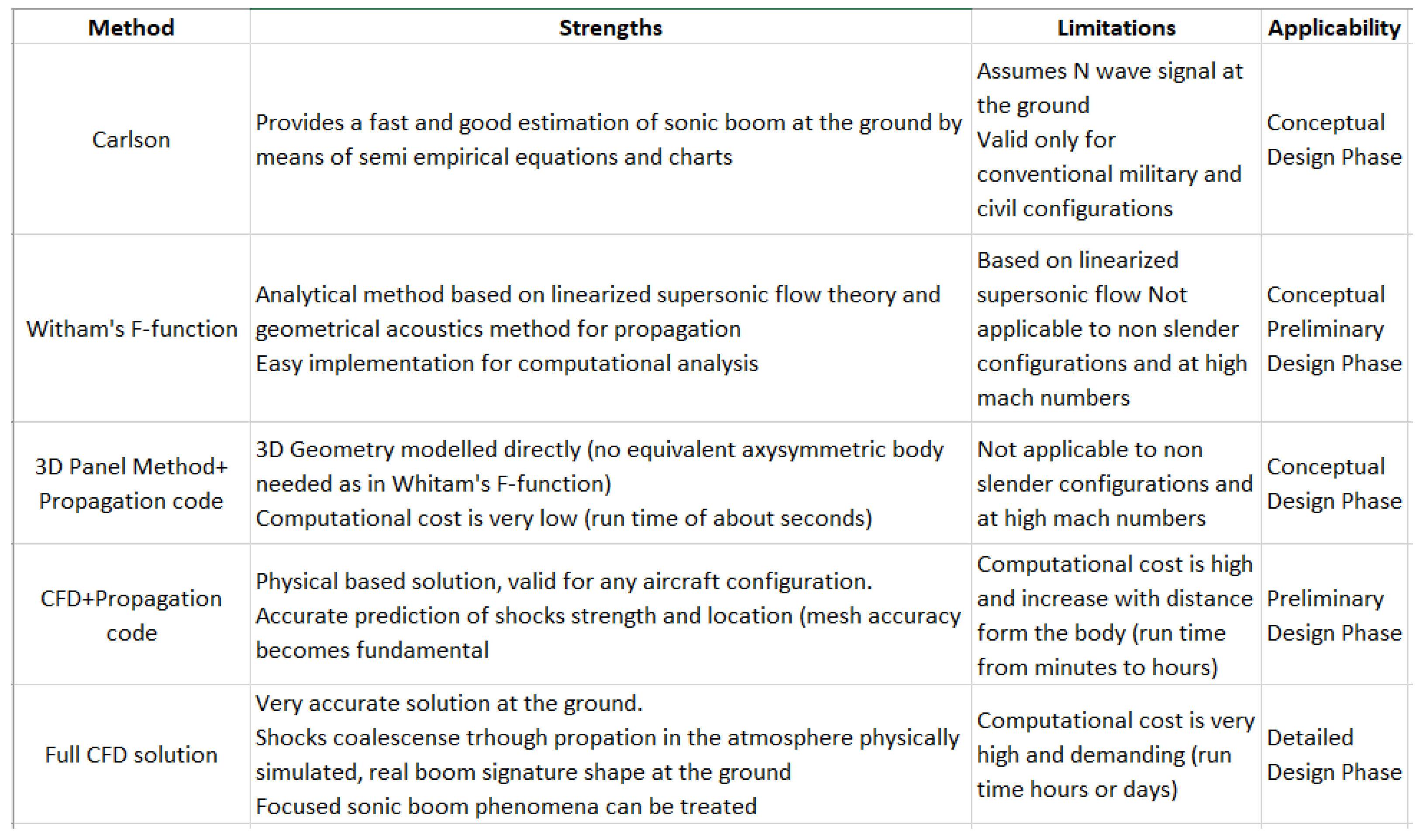
Figure 9. Review of sonic boom prediction methods.
Section 2.3, instead, provides an overview of the minimization techniques, developed over the years to shape the signal at the ground by optimally shaping the airframe. Sonic boom minimization is based on the Seebass–George–Darden (SGD) theory. According to this theory, given the flight conditions of altitude and Mach number and the aircraft parameters of weight and length, the equivalent area distribution needed to create either a minimum overpressure signature or a minimum shock signature can be mathematically defined. From the equivalent area distribution, the optimal aircraft shape can be easily found. The Shaped Sonic Boom Demonstration (SSBD) program successfully tested the low boom theory to be reliable under actual flight and atmospheric conditions. Further studies on this theory led to another technique to reduce the annoyance of the sonic boom on humans: the lobe-balancing technique. By trimming the lifting surfaces, a frozen shock balanced F-function could be generated, resulting in a less annoying multishock signature at the ground. These two minimization techniques have been used in several inverse design and optimization processes, where a target near-field or far-field pressure signature is achieved by careful aircraft shaping. Different optimization methods and algorithms can be used, such as the CFD adjoint-based and genetic algorithm.
However, though shaping the aircraft to reach the minimum sonic boom could effectively end in a low-boom aircraft configuration, it could lead to unfeasible solutions, especially in terms of cabin volume. In addition, the curved shaped body would strongly perturb the air stream flowing around the aircraft, affecting also aerodynamics. In the end, as already highlighted in the section, the low-boom requirements are in conflict with the low-drag requirements. A trade-off between these two fundamental requirements must be found in the next generation of supersonic aircraft, and this leads to not consider sonic boom minimization theories and techniques as a good solution.
References
- National Air and Space Museum. Available online: https://airandspace.si.edu/collection-objects/bell-x-1 (accessed on 18 October 2023).
- Gibbs, Y. Nasa Armstrong Fact Sheet: Sonic Booms. Available online: https://www.nasa.gov/centers/armstrong/news/FactSheets/FS-016-DFRC.html (accessed on 18 October 2023).
- Coulouvrat, F. The challenges of defining an acceptable sonic boom overland. In Proceedings of the 15th AIAA/CEAS Aeroacoustics Conference (30th AIAA Aeroacoustics Conference), Miami, FL, USA, 11–13 May 2009; p. 3384.
- Manci, K.M. Effects of Aircraft Noise and Sonic Booms on Domestic Animals and Wildlife: A Literature Synthesis; US Fish and Wildlife Service, National Ecology Research Center: Oxford, OH, USA, 1988; Volume 88.
- Darden, C.M. Sonic boom theory: Its status in prediction and minimization. J. Aircr. 1977, 14, 569–576.
- FAQBite. What is a Sonic Boom? Available online: https://faqbite.com/what/what-is-a-sonic-boom/ (accessed on 18 October 2023).
- Mabry, J.; Oncley, P. Establishing Certification/Design Criteria for Advanced Supersonic Aircraft Utilizing Acceptance, Interference, and Annoyance Response to Simulated Sonic Booms by Persons in Their Homes; Technical Report; Man-Acoustics And Noise Inc.: Seattle, WA, USA, 1973.
- Liu, S.R.; Tong, B. International Civil Aviation Organization Supersonic Task Group overview and status. J. Acoust. Soc. Am. 2017, 141, 3566.
- FAA. Supersonic Flight. Available online: https://www.faa.gov/newsroom/supersonic-flight?newsId=22754 (accessed on 18 October 2023).
- Plotkin, K.J. State of the art of sonic boom modeling. J. Acoust. Soc. Am. 2002, 111, 530–536.
- Abraham, T.A. Sonic Boom Loudness Reduction Through Localized Supersonic Aircraft Equivalent-Area Changes. Ph.D Thesis, Utah State University, Logan, UT, USA, 2021.
- Whitham, G.B. The flow pattern of a supersonic projectile. Commun. Pure Appl. Math. 1952, 5, 301–348.
- Whitham, G. On the propagation of weak shock waves. J. Fluid Mech. 1956, 1, 290–318.
- Hayes, W.D. Linearized supersonic flow. Ph.D Thesis, California Institute of Technology, Pasadena, CA, USA, 1947.
- Jones, R. Theory of Wing-Body Drag at Supersonic Speeds; (No. NACA-TR-1284); NASA: Washington, DC, USA, 1956.
- Whitcomb, R.T.; Fiscetti, T.L. Development of a Supersonic Area Rule and an Application to the Design of a Wing-Body Combination Having High Lift-to-Drag Ratios; (No. NACA-RM-L53H31a); NASA: Washington, DC, USA, 1953.
- Blokhintzev, D. The propagation of sound in an inhomogeneous and moving medium I. J. Acoust. Soc. Am. 1946, 18, 322–328.
- Carlson, H.W.; Maglieri, D.J. Review of sonic-boom generation theory and prediction methods. J. Acoust. Soc. Am. 1972, 51, 675–685.
- Lomax, H. The Wave Drag of Arbitrary Configurations in Linearized Flow as Determined by Areas and Forces in Oblique Planes; National Advisory Committee for Aeronautics: Hampton, VA, USA, 1955.
- Walkden, F. The shock pattern of a wing-body combination, far from the flight path. Aeronaut. Q. 1958, 9, 164–194.
- Carlson, H.W. An Investigation of Some Aspects of the Sonic Boom by Means of Wind-Tunnel Measurements of Pressures about Several Bodies at a Mach Number of 2.01; National Aeronautics and Space Administration: Hampton, VA, USA, 1959; Volume 161.
- Lina, L.J.; Maglieri, D.J. Ground Measurements of Airplane Shock-Wave Noise at Mach Numbers to 2.0 and at Altitudes to 60,000 Feet; National Aeronautics and Space Administration: Hampton, VA, USA, 1960; Volume 235.
- Smith, H.J. Experimental and Calculated Flow Fields Produced by Airplanes Flying at Supersonic Speeds; National Aeronautics and Space Administration: Hampton, VA, USA, 1960; Volume 621.
- Haefeli, R.; Hayes, W.; Kulsrud, H. Sonic Boom Propagation in a Stratified Atmosphere, with Computer Program; Technical Report; NASA: Hampton, VA, USA, 1969.
- THOMAS, C. Extrapolation of Sonic Boom Pressure Signatures by the Waveform Parameter Method (Extrapolation of Sonic Boom Pressure Signatures by Waveform Parameter Method and Comparison with F-Function Method); No. A-4232; NASA: Washington, DC, USA, 1972.
- Thomas, C.L. Extrapolation of Wind-Tunnel Sonic Boom Signatures without Use of a Whitham F-Function; NASA SP-255; NASA: Washington, DC, USA, 1970; pp. 205–217.
- Plotkin, K.J.; Downing, M.; Page, J. USAF single event sonic boom prediction model: PCBOOM. J. Acoust. Soc. Am. 1994, 95, 2839.
- Plotkin, K.J. Pcboom3 Sonic Boom Prediction Model-Version 1.0 c; Technical Report; Wyle Research Lab.: Arlington, VA, USA, 1996.
- George, A.; Plotkin, K. Sonic Boom Amplitudes and Waveforms in a Real Atmosphere. AIAA J. 1969, 7, 1978–1981.
- Carlson, H.W. Simplified Sonic-Boom Prediction; Technical Report; NASA: Hampton, VA, USA, 1978.
- Scarselli, G.; Marulo, F.; Averardo, M.; Cafiero, A.; Selmin, V. Numerical comparison between a siimplified method and a full CFD approach for sonic boom evaluation on supersonic innovative configurations. In Proceedings of the 13th AIAA/CEAS Aeroacoustics Conference (28th AIAA Aeroacoustics Conference), Southampton, UK, 14–17 June 2022; p. 3675.
- Clare, A.; Oman, R. Sonic Boom Prediction: A New Empirical Formulation and Animated Graphical Model. In Transformational Science And Technology For The Current And Future Force: (With CD-ROM); World Scientific: Singapore, 2006; pp. 565–572.
- Lee, R.; Downing, J. Sonic Booms Produced by United States Air Force and United States Navy Aircraft: Measured Data; Technical Report; Armstrong Lab.: Brooks Afb, TX, USA, 1991.
- Plotkin, K. Review of sonic boom theory. In Proceedings of the 12th Aeroacoustic Conference, San Antonio, TX, USA, 10–12 April 1989; p. 1105.
- McLean, F.E. Some Nonasymptotic Effects on the Sonic Boom of Large Airplanes; National Aeronautics and Space Administration: Hampton, VA, USA, 1965; Volume 2877.
- Jung, T.P.; Starkey, R.P.; Argrow, B. Modified linear theory sonic booms compared to experimental and numerical results. J. Aircr. 2015, 52, 1821–1837.
- Page, J.; Plotkin, K. An efficient method for incorporating computational fluid dynamics into sonic boom prediction. In Proceedings of the 9th Applied Aerodynamics Conference, Baltimore, MD, USA, 23–25 September 1991; p. 3275.
- Siclari, M.; Darden, C. Euler code prediction of near-field to midfield sonic boom pressure signatures. J. Aircr. 1993, 30, 911–917.
- Cheung, S.; Edwards, T.; Lawrence, S. Application of CFD to Sonic Boom Near and Mid flow-field prediction. In Proceedings of the 13th Aeroacoustics Conference, Washington, DC, USA, 5 June 1990; p. 3999.
- Cliff, S.E.; Thomas, S.D. Euler/experiment correlations of sonic boom pressure signatures. J. Aircr. 1993, 30, 669–675.
- Wintzer, M.; Ordaz, I. Under-Track CFD-Based Shape Optimization for a Low-Boom Demonstrator Concept. In Proceedings of the 33rd AIAA Applied Aerodynamics Conference, Dallas, TX, USA, 22–26 June 2015; p. 2260.
- Heath, C.M.; Slater, J.W.; Rallabhandi, S.K. Inlet trade study for a low-boom aircraft demonstrator. J. Aircr. 2017, 54, 1283–1293.
- Plotkin, K.; Page, J. Extrapolation of sonic boom signatures from CFD solutions. In Proceedings of the 40th AIAA Aerospace Sciences Meeting & Exhibit, Reno, NV, USA, 14–17 January 2002; p. 922.
- Rallabhandi, S.K.; Mavris, D.N. New computational procedure for incorporating computational fluid dynamics into sonic boom prediction. J. Aircr. 2007, 44, 1964–1971.
- Ordaz, I.; Li, W. Using CFD Surface Solutions to Shape Sonic Boom Signatures Propagated from Off-Body Pressure. In Proceedings of the 31st AIAA Applied Aerodynamics Conference, San Diego, CA, USA, 24–27 June 2013; p. 2660.
- Giblette, T.; Hunsaker, D.F. Prediction of sonic boom loudness using high-order panel methods for the near-field solution. In Proceedings of the AIAA Scitech 2019 Forum, San Diego, CA, USA, 7–11 January 2019; p. 0605.
- Ehlers, F.; Johnson, F.; Rubbert, P. A higher order panel method for linearized supersonic flow. In Proceedings of the 9th Fluid and PlasmaDynamics Conference, Williamsburg, VA, USA, July 1979; p. 381.
- Choi, S.; Alonso, J.J.; Kroo, I.M. Two-level multifidelity design optimization studies for supersonic jets. J. Aircr. 2009, 46, 776–790.
- Chan, M.K.Y. Supersonic Aircraft Optimization for Minimizing Drag and Sonic Boom; Stanford University: Stanford, CA, USA, 2003.
- Rallabhandi, S.; Mavris, D. Design and analysis of supersonic business jet concepts. In Proceedings of the 6th AIAA Aviation Technology, Integration and Operations Conference (ATIO), Wichita, KS, USA, 25–27 September 2006; p. 7702.
- Ueno, A.; Kanamori, M.; Makino, Y. Multi-fidelity low-boom design based on near-field pressure signature. In Proceedings of the 54th AIAA Aerospace Sciences Meeting, San Diego, CA, USA, 4–8 January 2016; p. 2033.
- Rallabhandi, S.K. Advanced sonic boom prediction using the augmented Burgers equation. J. Aircr. 2011, 48, 1245–1253.
- Cleveland, R.O. Propagation of Sonic Booms through a Real, Stratified Atmosphere. Ph.D. Thesis, The University of Texas at Austin, Austin, TX, USA, 1995.
- Robinson, L.D. Sonic Boom Propagation through an Inhomogeneous, Windy Atmosphere. Ph.D. Thesis, The University of Texas at Austin, Austin, TX, USA, 1991.
- Pilon, A.R. Spectrally accurate prediction of sonic boom signals. AIAA J. 2007, 45, 2149–2156.
- Lonzaga, J.B. Recent Enhancements to NASA’ s PCBoom Sonic Boom Propagation Code. In Proceedings of the AIAA Aviation 2019 Forum, Dallas, TX, USA, 17–21 June 2019; p. 3386.
- Yamamoto, M.; Hashimoto, A.; Aoyama, T.; Sakai, T. A unified approach to an augmented Burgers equation for the propagation of sonic booms. J. Acoust. Soc. Am. 2015, 137, 1857–1866.
- Ozcer, I. Sonic boom prediction using Euler/full potential methodology. In Proceedings of the 45th AIAA Aerospace Sciences Meeting and Exhibit, Reno, NV, USA, 8–11 January 2007; p. 369.
- Stout, T.A. Simulation of N-Wave and Shaped Supersonic Signature Turbulent Variations. Ph.D. Thesis, The Pennsylvania State University, State College, PA, USA, 2018.
- Crow, S. Distortion of sonic bangs by atmospheric turbulence. J. Fluid Mech. 1969, 37, 529–563.
- Pierce, A.D. Statistical theory of atmospheric turbulence effects on sonic-boom rise times. J. Acoust. Soc. Am. 1971, 49, 906–924.
- Pierce, A.D.; Maglieri, D.J. Effects of atmospheric irregularities on sonic-boom propagation. J. Acoust. Soc. Am. 1972, 51, 702–721.
- Plotkin, K.J.; George, A. Propagation of weak shock waves through turbulence. J. Fluid Mech. 1972, 54, 449–467.
- Blanc-Benon, P.; Lipkens, B.; Dallois, L.; Hamilton, M.F.; Blackstock, D.T. Propagation of finite amplitude sound through turbulence: Modeling with geometrical acoustics and the parabolic approximation. J. Acoust. Soc. Am. 2002, 111, 487–498.
- Averiyanov, M.; Blanc-Benon, P.; Cleveland, R.O.; Khokhlova, V. Nonlinear and diffraction effects in propagation of N-waves in randomly inhomogeneous moving media. J. Acoust. Soc. Am. 2011, 129, 1760–1772.
- Bradley, K.A.; Hobbs, C.M.; Wilmer, C.B.; Sparrow, V.W.; Stout, T.A.; Morgenstern, J.M.; Underwood, K.H.; Maglieri, D.J.; Cowart, R.A.; Collmar, M.T.; et al. Sonic Booms in Atmospheric Turbulence (SONICBAT): The Influence of Turbulence on Shaped Sonic Booms; (No. NASA/CR–2020–220509); NASA: Washington, DC, USA, 2020.
- Locey, L.L. Sonic Boom Postprocessing Functions to Simulate Atmospheric Turbulence Effects; The Pennsylvania State University: State College, PA, USA, 2008.
- Luquet, D. 3D Simulation of Acoustical Shock Waves Propagation through a Turbulent Atmosphere. Application to Sonic Boom. Ph.D Thesis, Université Pierre et Marie Curie, Paris, France, 2016.
- Dagrau, F.; Rénier, M.; Marchiano, R.; Coulouvrat, F. Acoustic shock wave propagation in a heterogeneous medium: A numerical simulation beyond the parabolic approximation. J. Acoust. Soc. Am. 2011, 130, 20–32.
- Kanamori, M.; Takahashi, T.; Naka, Y.; Makino, Y.; Takahashi, H.; Ishikawa, H. Numerical Evauation of Effect of Atmospheric Turbulence on Sonic Boom Observed in D-SEND# 2 Flight Test. In Proceedings of the 55th AIAA Aerospace Sciences Meeting, Grapevine, TX, USA, 9–13 January 2017; p. 0278.
- Kanamori, M.; Takahashi, T.; Ishikawa, H.; Makino, Y.; Naka, Y.; Takahashi, H. Numerical Evaluation of Sonic Boom Deformation due to Atmospheric Turbulence. AIAA J. 2021, 59, 972–986.
- Leconte, R.; Marchiano, R.; Coulouvrat, F.; Chassaing, J.C. Influence of atmospheric turbulence parameters on the propagation of sonic boom. In Proceedings of the Forum Acusticum, Lyon, France, 7–11 December 2021; pp. 979–980.
- Kandil, O.; Ozcer, I.; Khasdeo, N. Sonic Boom Prediction, Focusing, and Mitigation. In Proceedings of the 2S Congress of the Aeronautical Sciences 2006, Hamburg, Germany, 3–8 September 2006.
- Griffiths, G.W.; Schiesser, W.E. Linear and nonlinear waves. Scholarpedia 2009, 4, 4308.
- Van Hove, B.; Lofqvist, M.; Bonetti, D.; Kokorich, M. Reducing the Noise of Hypersonic Aircraft. 2023. Available online: https://www.researchgate.net/publication/367966282_Reducing_the_Noise_of_Hypersonic_Aircraft (accessed on 18 October 2023).
- Guiraud, J.P. Acoustique geometrique bruit balistique des avions supersoniques et focalisation. J. Mec. 1965, 4, 215.
- Seebass, R. Nonlinear Acoustic Behavior at a Caustic; Technical Report; Boeing Scientific Research Labs.: Seattle, WA, USA, 1971.
- Gill, P.; Seebass, A. Nonlinear Acoustic Behavior at a Caustic-An Approximate Analytical Solution. In Aeroacoustics: Fan; MIT Press: Cambridge, MA, USA, 1975; pp. 353–386.
- Plotkin, K.; Cantril, J. Prediction of sonic boom at a focus. In Proceedings of the 14th Aerospace Sciences Meeting, Washington, DC, USA, 26–28 January 1976; p. 2.
- Marchiano, R.; Coulouvrat, F.; Grenon, R. Numerical simulation of shock wave focusing at fold caustics, with application to sonic boom. J. Acoust. Soc. Am. 2003, 114, 1758–1771.
- Auger, T.; Coulouvrat, F. Numerical simulation of sonic boom focusing. AIAA J. 2002, 40, 1726–1734.
- Kandil, O.; Zheng, X. Prediction of Superboom Problem Using Computational Solution of Nonlinear Tricomi Equation. In Proceedings of the AIAA Atmospheric Flight Mechanics Conference and Exhibit, San Francisco, CA, USA, 15–18 August 2005; p. 6335.
- Kandil, O.; Zheng, X. Computational solution of nonlinear Tricomi equation for sonic boom focusing and applications. In Proceedings of the AIP Conference Proceedings. American Institute of Physics, Mexico City, Mexico, 10–14 July 2006; Volume 838, pp. 607–610.
- Piacsek, A.A. A Numerical Study of Weak Step Shocks That Focus in Two Dimensions. Ph.D. Thesis, The Pennsylvania State University, State College, PA, USA, 1995.
- Piacsek, A.A. Atmospheric turbulence conditions leading to focused and folded sonic boom wave fronts. J. Acoust. Soc. Am. 2002, 111, 520–529.
- Loubeau, A. Recent progress on sonic boom research at NASA. In Proceedings of the INTER-NOISE and NOISE-CON Congress and Conference Proceedings. Institute of Noise Control Engineering, New York City, NY, USA, 19–22 August 2012; Volume 2012, pp. 3760–3770.
- Taylor, A.D. The TRAPS Sonic Boom Program; Department of Commerce, National Oceanic and Atmospheric Administration: Washington, DC, USA, 1980; Volume 87.
- Rallabhandi, S.; Fenbert, J. Numerical simulation of sonic boom focusing and its application to mission performance. J. Acoust. Soc. Am. 2017, 141, 3566.
- E. U. Rumble. H2020. Available online: https://rumble-project.eu/i/dissemination/conference-presentations (accessed on 18 October 2023).
- Töpken, S.; van de Par, S. Loudness and short-term annoyance of sonic boom signatures at low levels. J. Acoust. Soc. Am. 2021, 149, 2004–2015.
- Marshall, A.; Davies, P. A semantic differential study of low amplitude supersonic aircraft noise and other transient sounds. In Proceedings of the International Congress on Acoustics, Madrid, Spain, 2–7 September 2007; pp. 1–6.
- Marshall, A.; Davies, P. A comparison of perceptual attributes and ratings of environmental transient sounds in two different playback environments. In Proceedings of the INTER-NOISE and NOISE-CON Congress and Conference Proceedings. Institute of Noise Control Engineering, Shanghai, China, 26–29 October 2008; Volume 2008, pp. 5586–5592.
- Marshall, A.; Davies, P. Metrics including time-varying loudness models to assess the impact of sonic booms and other transient sounds. Noise Control. Eng. J. 2011, 59, 681–697.
- Glasberg, B.R.; Moore, B.C. A model of loudness applicable to time-varying sounds. J. Audio Eng. Soc. 2002, 50, 331–342.
- Zwicker, E.; Fastl, H. Psychoacoustics: Facts and Models; Springer Science & Business Media: Berlin, Germany, 2013; Volume 22.
- Maglieri, D.J.; Huckel, V.; Henderson, H.R. Variability in Sonic Boom Signatures Measured Along an 8000-Foot Linear Array; National Aeronautics and Space Administration: Washington, DC, USA, 1969; Volume 5040.
- Doebler, W.J.; Sparrow, V.W. Stability of sonic boom metrics regarding signature distortions from atmospheric turbulence. J. Acoust. Soc. Am. 2017, 141, EL592–EL597.
- Leatherwood, J.D.; Sullivan, B.M. Loudness and Annoyance Response to Simulated Outdoor and Indoor Sonic Booms; No. NASA-TM-107756; NASA: Washington, DC, USA, 1993.
- Stevens, S.S. Perceived level of noise by Mark VII and decibels (E). J. Acoust. Soc. Am. 1972, 51, 575–601.
- Borsky, P.N.; York, N.O.R.C.N. Community Reactions to Sonic Booms in the Oklahoma City Area: Volume 2. Data on Community Reactions and Interpretations; Aerospace Medical Research Laboratories: Brooks AFB, TX, USA, 1965.
- Clarkson, B.L.; Mayes, W.H. Sonic-Boom-Induced Building Structure Responses Including Damage. J. Acoust. Soc. Am. 1972, 51, 742–757.
- Sizov, N.V.; Plotkin, K.J.; Hobbs, C.M. Predicting transmission of shaped sonic booms into a residential house structure. J. Acoust. Soc. Am. 2010, 127, 3347–3355.
- Minelli, A. Aero-Acoustic Shape Optimization of a Supersonic Business Jet. Ph.D. Thesis, Université Nice Sophia Antipolis, Nice, France, 2013.
- Jones, L. Lower bounds for sonic bangs. Aeronaut. J. 1961, 65, 433–436.
- Carlson, H.W. The Lower Bound of Attainable Sonic-Boom Overpressure and Design Methods of Approaching This Limit; National Aeronautics and Space Administration: Washington, DC, USA, 1962.
- Carlson, H.W. Influence of airplane configuration on sonic-boom characteristics. J. Aircr. 1964, 1, 82–86.
- Darden, C.M.; Powell, C.A.; Hayes, W.D.; George, A.R.; Pierce, A.D. Status of sonic boom methodology and understanding. In Proceedings of the Sonic Boom Workshop, Hampton, VA, USA, 1 June 1989.
- George, A.; Seebass, R. Sonic boom minimization including both front and rear shocks. AIAA J. 1971, 9, 2091–2093.
- Seebass, R.; George, A.R. Sonic-Boom Minimization. J. Acoust. Soc. Am. 1972, 51, 686–694.
- Darden, C.M. Sonic-Boom Minimization with Nose-Bluntness Relaxation; National Aeronautics and Space Administration, Scientific and Technical: Washington, DC, USA, 1979; Volume 1348.
- Carlson, H.W.; Barger, R.L.; Mack, R.J. Application of Sonic-Boom Minimization Concepts in Supersonic Transport Design; No. NASA-TN-D-7218; NASA: Washington, DC, USA, 1973.
- Mack, R.J. Wind-Tunnel Investigation of the Validity of a Sonic-Boom-Minimization Concept; NASA TP D-1421; NASA: Washington, DC, USA, 1979.
- Mack, R.J.; Needleman, K.E. A Methodology for Designing Aircraft to Low Sonic Boom Constraints; Technical Report; NASA: Washington, DC, USA, 1991.
- Rallabhandi, S.K.; Mavris, D.N. Aircraft geometry design and optimization for sonic boom reduction. J. Aircr. 2007, 44, 35–47.
- Plotkin, K.; Rallabhandi, S.; Li, W. Generalized formulation and extension of sonic boom minimization theory for front and aft shaping. In Proceedings of the 47th AIAA Aerospace Sciences Meeting including The New Horizons Forum and Aerospace Exposition, Orlando, FL, USA, 5–8 January 2009; p. 1052.
- Jung, T.P.; Starkey, R.P.; Argrow, B. Lobe balancing design method to create frozen sonic booms using aircraft components. J. Aircr. 2012, 49, 1878–1893.
- Farhat, C.; Argrow, B.; Nikbay, M.; Maute, K. Shape optimization with F-function balancing for reducing the sonic boom initial shock pressure rise. Int. J. Aeroacoustics 2004, 3, 361–377.
- Minelli, A.; Salah el Din, I.; Carrier, G. Inverse design approach for low-boom supersonic configurations. AIAA J. 2014, 52, 2198–2212.
- Wintzer, M.; Kroo, I.; Aftosmis, M.; Nemec, M. Conceptual design of low sonic boom aircraft using adjoint-based CFD. In Proceedings of the Seventh International Conference on Computational Fluid Dynamics (ICCFD7), Big Island, HI, USA, 9–13 July 2012.
- Feng, X.; Li, Z.; Song, B. Research of low boom and low drag supersonic aircraft design. Chin. J. Aeronaut. 2014, 27, 531–541.
- Li, W.; Rallabhandi, S. Inverse design of low-boom supersonic concepts using reversed equivalent-area targets. J. Aircr. 2014, 51, 29–36.
- Zhang, Y.; Huang, J.; Zhenghong, G.; Chao, W.; Bowen, S. Inverse design of low boom configurations using proper orthogonal decomposition and augmented Burgers equation. Chin. J. Aeronaut. 2019, 32, 1380–1389.
- Li, W.; Geiselhart, K. Multidisciplinary design optimization of low-boom supersonic aircraft with mission constraints. AIAA J. 2021, 59, 165–179.
More
Information
Subjects:
Engineering, Aerospace
Contributors
MDPI registered users' name will be linked to their SciProfiles pages. To register with us, please refer to https://encyclopedia.pub/register
:
View Times:
2.9K
Revisions:
3 times
(View History)
Update Date:
08 Nov 2023
Table of Contents


Notice
You are not a member of the advisory board for this topic. If you want to update advisory board member profile, please contact office@encyclopedia.pub.
OK
Confirm
Only members of the Encyclopedia advisory board for this topic are allowed to note entries. Would you like to become an advisory board member of the Encyclopedia?
Yes
No
${ textCharacter }/${ maxCharacter }
Submit
Cancel
Back
Comments
${ item }
|
${ item.createdUser.fullName }
${ item.createdAt }
${ item.vote }
${ item.reply }
Delete
${ reply.createdUser.fullName }
${ reply.createdAt }
${ reply.vote }
Delete
There is no reply to this comment~
${ item.replyTextCharacter }/${ item.replyMaxCharacter }
Submit
Cancel
More
No more~
There is no comment~
${ textCharacter }/${ maxCharacter }
Submit
Cancel
${ selectedItem.replyTextCharacter }/${ selectedItem.replyMaxCharacter }
Submit
Cancel
Confirm
Are you sure to Delete?
Yes
No