Machine Learning for Hydropower Generation

Version	Summary	Created by	Modification	Content Size	Created at	Operation
1		Sara Séguin	--	3508	2023-06-26 22:30:30	\|
2	Reference format revised.	Lindsay Dong	Meta information modification	3508	2023-06-27 03:02:41	\|

This entry is adapted from the peer-reviewed paper 10.3390/en16083335

Hydropower is the most prevalent source of renewable energy production worldwide. As the global demand for robust and ecologically sustainable energy production increases, developing and enhancing the current energy production processes is essential. In the past decade, machine learning has contributed significantly to various fields, and hydropower is no exception. All three horizons of hydropower models could benefit from machine learning: short-term, medium-term, and long-term. Dynamic programming is used in the majority of hydropower scheduling models.

hydropower hydropower scheduling machine learning

1. Introduction

Hydropower generation is a complex problem that needs to be defined in its many aspects in order to have a good grasp of how models are built in this field ^[1]^[2]^[3]. The publication of ^[4] aims to survey the various research advances in hydropower generation while providing a detailed description of the optimization process over a short, medium, and long-term horizon.

The scholars of ^[2] looked at how machine learning has been used to address the issue of reservoir inflow during the past decade, but they did not look at the most recent models. The scholars of the same work covered modeling principles for hydroelectric plants. They also presented the underlying methodology of hydropower generation and the concerns that need to be considered while developing a decision model within this context.

There are three different kinds of hydroelectric power plants: run-of-river, pumped storage, and reservoirs (which are large dams). The majority of hydroelectric power facilities that generate electricity are of the reservoir variety. This power plant is situated in close proximity to a dam, which serves as a reservoir for water that is used to control the amount of electricity produced by the facility.

A reservoir gives the power plant the ability to control the amount of water that is consumed. Because of this characteristic, the power plant’s energy production is very adaptable ^[5], and as a result, it can better satisfy demands for electricity.

The production of electricity at run-of-river power plants does not require the use of a reservoir because the plants instead rely on the flow of the river.

The lack of a reservoir makes it impossible to maintain a consistent water level, which results in a high rate of overflow in these rivers and lakes. Because of this, the amount of power produced is highly dependent on the intensity of the current and the volume of water entering the penstock. The impact of the climate also plays an important role in the production, as in the model of ^[6].

Reservoir power plants and pumped-storage power plants both function by storing energy in a reservoir. The key distinction is that the water is collected in a reservoir that is positioned downstream after it has been processed by the power plant. This reservoir is connected to the reservoir upstream of it by a pipe, and as a result, it is possible to pump water from the lower reservoir into the upper reservoir. This power plant acts in a manner analogous to that of a battery and is used to store excess energy ^[7]. As a result of the fact that these plants are not connected to a watershed, they are unable to generate any additional electricity.

The pumped-storage power plant is the most cost-effective energy storage method, with an energy retention efficiency of around 80%. It is Europe’s most common energy storage method ^[8]. This infrastructure can also be coupled with intermittent energy sources, such as the hydro-wind power plant in El Hierro, which allows the storage of additional energy produced by the nearby offshore wind farm ^[9].

2. Hydropower Scheduling Models

When optimizing hydroelectric power facilities, the goal is often to increase the amount of energy produced by the plant while simultaneously increasing the amount of money made from selling that energy. On the other hand, it is much more frequent in the optimization model research to concentrate on efficiency and/or profit.

As a result of the fixed price of electricity that is imposed by a state-owned company in Canada and Quebec in particular, the models that are developed in this region tend to place a greater emphasis on energy production. This is caused by the management of hydroelectricity by the government enterprise Hydro-Québec.

Private enterprises in other parts of the United States and Europe are in charge of the generation of hydroelectric power; these businesses’ primary objective is to sell their hydroelectric output to the highest potential buyer.

This strategy is supported by the scholars ^[10] on the grounds that it reduces production costs while maintaining a high level of reliability. Typically, the sale of electricity is conducted through an auction in which producers put offers based on their production costs and purchasers place bids depending on their consumption needs.

In this economic setting, the purpose of these models is to maximize profit from the sale of energy produced. There are a number of ways to calculate the price of energy produced per hour, including those proposed by ^[10].

Most models take into account the operational costs of the plant when optimizing for profit. For example, this can be represented in short-term optimization by the starting and stopping of turbine units, or in the long term by breaking even with the expense of the plants. In older hydro plants, maintenance of generator units may even require its own optimization model, since maintenance occurs quite frequently and can easily offset energy production if not carried out properly ^[11].

There are also hydroelectric systems operated by energy-intensive industries, such as the Rio Tinto facility that operates the Saguenay Lac-Saint-Jean hydroelectric system. These companies have set electricity needs, which makes the unpredictability of the power plants in relation to the need for energy output more adaptable.

A hydroelectric power plant is frequently connected to other power plants located upstream and downstream. This is referred to as a hydroelectric system, which may include numerous reservoirs, powerplants, and run-of-river powerplants along interconnected rivers and lakes.

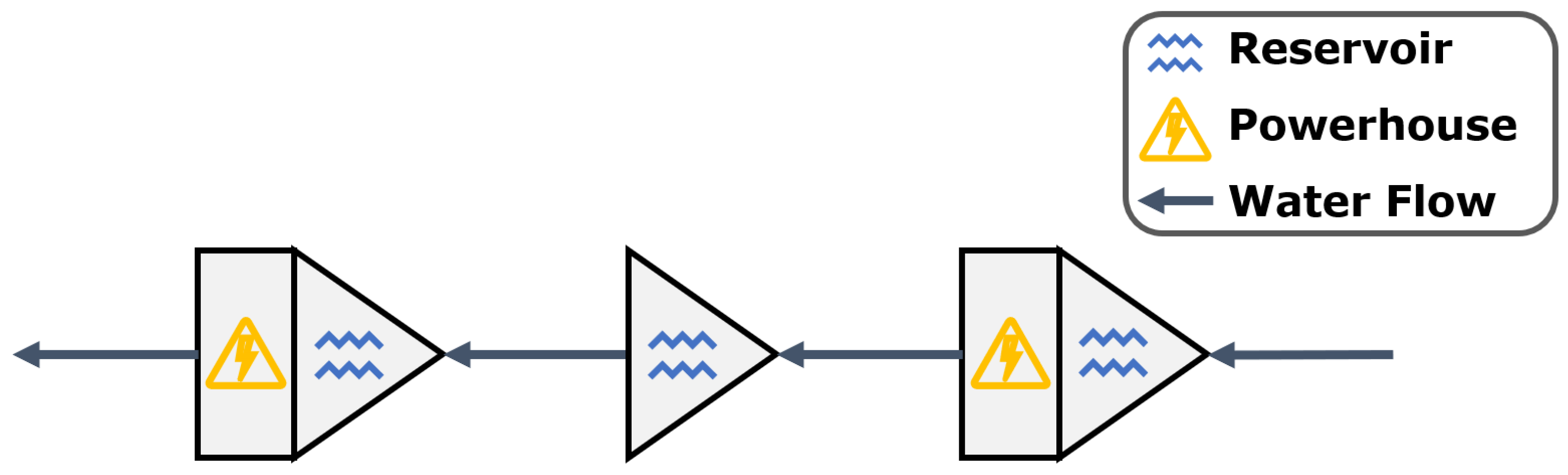
The illustration depicting a cascade system is shown in Figure 1. Each hydroelectric plant is situated within a watershed, from which water will ultimately flow into one of the territory’s reservoirs. Hydrology is the study of the distribution, flow, and quality of water, as described in detail by ^[12].

/media/item_content/202306/649a33aa9fc4aenergies-16-03335-g001.png

Figure 1. An example of a hydropower system with three reservoirs and two powerhouses. The arrow shows the direction of water movement, which can be held and released when interacting with a reservoir (triangle) and a powerhouse (rectangle).

In the field of optimization, the quality of a model is frequently judged based on how accurately it predicts the amount of water that will be added to a system.

2.1. Approximating Hydropower Production

A nonlinear and non-convex function represents the power produced by a turbine in a hydroelectric facility. This sort of function is far more difficult to optimize than its linear convex equivalents.

Depending on their complexity, nonlinear functions can be more challenging to work with, but the non-convexity of the production function is the fundamental issue in mathematical optimization. However, it is still possible to design non-convex optimization models, such as ^[13], who experimented with a medium-term model. In addition, they observed that this form of model soon becomes computationally expensive as the size of the problem increases, particularly when constraints are added to their model. In addition, the performance improvement is deemed insufficient to warrant the increase in computing time.

The scholars in ^[14] evaluate the linearization of a nonlinear mixed integer model. The transformation from a nonlinear function to a linear one improves the efficiency of the resolution time but necessarily causes a loss of the precision of the results.

On the other hand, adopting a mixed integer linear programming model has enabled the addition of various constraints, mitigates the losses associated with the linear approximation, and permits an increase in the problem’s complexity.

2.2. Scenario Tree

Water inflows are unpredictable in hydropower. Because of this, it is hard to anticipate with accuracy the water level in the reservoirs. Despite the fact that a turbine’s electrical energy output is reliant on the water level in the reservoir, it is nevertheless feasible to achieve fully ideal hydroelectric production. This is accomplished by constructing a scenario tree of the anticipated influx. This is why stochastic models are frequently mentioned in the literature on hydropower. A stochastic model contains at least one uncertain variable.

In order to predict water inflows for power generation purposes, the scholars in ^[15] address the problem in a short-term optimization model. To predict hydroelectric generation, a scenario tree structure is used. They investigate and analyze, among other things, three strategies for estimating the input scenario on the production of the hydroelectric system in the Saguenay region, Quebec, Canada.

Using a black-box optimization solver, the first method identifies the set of scenario trees that maximizes energy production. The scenario tree has three input parameters: the number of stages, the number of child nodes for each node, and the aggregation level for each day. The scenario tree is optimized to maximize hydroelectric production by returning water flows, reservoir volume, and working turbines based on the output of an input scenario.

Another model uses this last result to maximize the number of turbines by restricting each turbine’s start-up and shut-down times. Each day, a new scenario tree is constructed based on meteorological data, and the water level in the reservoir is computed. The second approach employs the median scenario determined by the black box, whereas the third method, scenario fans, allows only the tree’s root to have several child nodes.

3. Machine Learning in Hydropower Production

This tendency toward employing machine learning models for predicting inflow is a consequence of the complexity inherent in simulating the water leveling process using conventional model methods. The behavior of water is influenced by a number of stochastic and natural resources, including inflows from upstream river reservoirs, evaporation from the reservoir surface, temperature variations, and other environmental factors ^[16].

Since most of the works focus on predicting water inflows to reservoirs, the scholar explores the application of machine learning to Cyber-Physical Systems.

3.1. Linear Regression

A Linear Regression (LR) model is a technique for predicting the type of function based on the relationship between two or more data elements. Typically, the purpose is to decrease the value of a cost function associated with each point’s distance. This is accomplished by employing a “closed-form” equation that directly computes the model parameters that best suit the model.

However, a high number of features and instances may necessitate using a gradient descent method to optimize the cost function ^[17]. Despite this, these models are renowned for their simplicity and speed of computation.

A study in ^[18] examines 30 years of water input over an extended time frame (one year per instance). Their objective is to create a prediction model of annual water inflows for a hydropower plant—collecting and standardizing data for each place within the dataset.

The results demonstrate that the model can estimate the trend of plants separated by rivers. When a period contains fewer than 30 years, the model is especially sensitive to outliers.

The emphasis of the work in ^[19] is creating a strategy for forecasting the change in the annual hydroelectric output of federal hydroelectric plants in the United States. This method is based on the correlation between geological runoff data and the yearly hydroelectric production of 132 U.S. plants.

Monthly data collection occurred between 1989 and 2008, spanning a period of twenty-nine years. Three types of projection models are utilized: global, regional, and local. The data indicate that the correlation between runoff and hydropower production is increasing, with an overall tendency toward a dryer climate.

A seasonal runoff projection model is used by looking at each season separately. Seasons are separated by a three-month interval, starting in spring (March). Trend seems to vary a lot based on the region observed.

The linear regression data were utilized to forecast the change in production till 2039. This forecast offers fresh perspectives on annual and seasonal production that might be utilized in future endeavors.

Predicting the water level in a reservoir used by a hydroelectric plant using two different scenarios over a relatively short time horizon is the purpose of the research presented in the publication cited ^[16].

In the first scenario, there is rainfall and water level. In contrast, in the second scenario, there is precipitation, water level, and water release from a power plant.

Four machine learning methods were tested in ^[16]: Boosted Decision Tree Regression, Decision Forest Regression, Bayesian Linear Regression, and Neural Network Regression.

When looking at the results on a Taylor diagram and comparing them with other machine learning performance metrics (MAE, MSE, RMSE,

R^{2}

, and RAE), the Bayesian Linear Regression approach produces the best overall outcomes.

The 12531 data set containing 34 years of daily water level and precipitation data was harvested from 1985 to 2019, and 82,057 h set was recorded between 2010 and 2019. The results show that all methods are suitable for water level prediction, but Bayesian Linear Regression is particularly effective for the first scenario and Boosted Decision Tree Regression for the second scenario.

The scholars in ^[20] discuss the creation of many medium-term regressive models (monthly and quarterly) to anticipate the amount of energy produced by a hydroelectric plant.

Four types of regressive algorithms include power regression, multiple linear regression, Gaussian process regression, and support vector regression. The precipitation data in this set spans a period of 26 years, from 1993 to 2019, and was collected from six different locations.

The information that was utilized refers to the amount of rainfall, temperature, and evaporation that occurred from the plant reservoir. According to the findings, the Gaussian process regression model is superior to the other approaches in terms of performance.

Gaussian refers to a method that is defined by the means and standard deviation; this method does not require any parameters, is appropriate for use with small datasets, and is able to take into account the uncertainty of the predictions.

By employing this model, the scholars in ^[20] could establish a connection between the weather forecast and the amount of power the plant generated. According to the scholars, monthly data are not ideal for forecasting energy generation; instead, quarterly precipitation generates the most accurate projections with a high correlation. In recent research, there appears to be an abundance of regressive algorithms, necessitating testing the same problem on each approach to derive the model.

Despite the simplicity of this type of procedure, the findings achieved with this instrument are generally of high quality. However, regressive algorithms can only supply limited information.

In general, the result of the predictions made by this class of algorithms reveals more information about the situation, allowing for a more precise examination of the projected data. On a bigger scale, linear regression algorithms appear better suited as complementary to more advanced machine learning algorithms with a broader definition of the hydropower production problem.

3.2. Random Forest

A decision tree is a type of machine learning algorithm that is able to perform tasks involving classification as well as regression. The scholars in ^[17] develop a model with the help of a labelled dataset by basing their decisions on the characteristics of the input data. They are the fundamental building blocks of the Random Forest (RF) model, which is one of the most effective machine learning algorithms.

According to the scholars in ^[21], in comparison to linear regression models, random forest makes use of ensemble learning by constructing a large number of distinct trees. These trees are then used to make many predictions based on an input and to provide a more accurate inference from the variables.

The bagging method is often described as the main reason as to why ensemble methods work so well in the random forest algorithm. This is done by training the decision trees of a random forest with a slightly different subset of a training set in order to obtain a different prediction each time ^[22].

Observing the links between market price and inflows and labeling each feature as stochastic or deterministic in order to construct a model that classifies each occurrence as deterministic or random.

The second regression model is trained to forecast a decision heuristic for determining if a deterministic approach should be employed for the current market. The dataset was altered to obtain more accurate predictions. By comparing the performance of some data to the market price, the strategy gap function was introduced. To examine the relationships between the features in the set, a correlation matrix with Spearman’s coefficient was generated.

No feature reduction was undertaken based on the results of test models. The gradient boosting decision tree approach was employed as the random forest algorithm ^[23].

The selection of the model’s hyperparameters was based on 1000 random parameter selections applied to five random sets. The performance of the models was determined by calculating the accurate classification rate based on the total number of classifications conducted, the performance gap, and the average performance of an optimal design.

3.3. Reinforcement Learning

Environment and state are defined in the context of hydropower production by the data produced by power plants and their reservoirs. A policy can be represented in a variety of ways.

In the paper by ^[24], a deep reinforcement learning method is used to optimize a cascade power plant network located on the Hun River in northern China. Specifically, these use the Deep Q-Network method, introduced in ^[25], as a prediction model and use a Bayesian aggregation–disaggregation technique on the three reservoirs to reduce the dimensionality of the problem.

The DRL consists of an agent with two neural networks as its brain (an action and a target network), allowing it to make decisions regarding its surroundings. The environment is represented by the dataset of hydroelectric power facilities. From 1967 to 2015, the statistics include daily precipitation and 10-day inflows for each reservoir.

After receiving information on the condition of its surroundings, the agent decides whether or not to utilize the DQN’s network capabilities. The model will mimic this activity in order to return a reward to the agent based on the divergence of the system’s needs and the amount of energy that was produced. The agent retains all of its previous states, actions, and rewards so that it can engage in continuous learning.

The DRL model is compared using three Stochastic Dynamic Programming (SDP) models. The methods using DRL are said to be better than their SDP counterparts, but few conclusions are made from this point of view, and the graphs seem to show similar results between the two methods.

The scholar makes note of the fact that DRL with memory is applicable to the real-time production problem, and that Bayesian aggregation–disaggregation appears to be appropriate to the problem of cascading tank systems. Both of these points are taken into consideration.

The paper ^[26] uses DRL on a long-term horizon problem to optimize annual revenues based on water inflow and electricity prices. The reinforcement algorithm is of type actor-critic with a Q-learning algorithm.

The water level inside a reservoir symbolizes the environment, and the agent’s goal is to achieve a state of equilibrium in the reservoir’s water level to minimize the amount of water that spills out and increase the amount of money the agent makes each week.

The activity that needs to be completed by the agent is to determine, based on the current price of power on the market, what percentage of the water in the tank should be converted into energy.

The reward function for action is computed with respect to the greatest capacity of power that can be produced in proportion to the reservoir’s capacity, the electricity price on a weekly basis, and the importance connected to this price. All of these factors are taken into account.

The critic is composed of four neural networks, including a network describing the value of the state, a target network allowing a better convergence of the error backpropagation algorithm, and two Q-networks to obtain the Q value.

The decisions that the actor makes are determined by a neural network designed to represent the policies in place in the state. It is important to emphasize using RMSprop to optimize their network, which is one of the hyperparameters.

This decision was made because, compared to Adam, it has less momentum dependence when applied to non-stationary data and a constantly shifting environment. In addition, using RMSprop helps to level out the differences in learning rates and prevents an excessive investigation into a local minimum.

The model is trained on an artificial scenario set in addition to a scenario set developed using data from 2008 to 2019 on European Nordic market value data from 1958 to 2019 on Norwegian water supply, and four reservoirs with comparable meteorological conditions. The model converges after one day of training with 300,000 weeks on a processor with 3.1 GHz and 16 GB of RAM ^[26].

The work demonstrates the viability of a reinforcement-based model in a minimalist hydroelectric generation problem from the perspective of the field in which hydroelectric optimization models dominate. Specifically, this is done by looking at the problem from the point of view of the hydroelectric optimization models. The scholar incorporates the option of pushing the model farther with the use of algorithms such as aggregation–disaggregation ^[26].

References

British Petroleum Corporate Communications Services British Petroleum Statistical Review of World Energy; British Petroleum Corporate Communications Services: London, UK, 2021.
Bordin, C.; Skjelbred, H.I.; Kong, J.; Yang, Z. Machine Learning for Hydropower Scheduling: State of the Art and Future Research Directions. Procedia Comput. Sci. 2020, 176, 1659–1668.
Sun, S.; Cao, Z.; Zhu, H.; Zhao, J. A Survey of Optimization Methods From a Machine Learning Perspective. IEEE Trans. Cybern. 2020, 50, 3668–3681.
Benkalai, I.; Séguin, S. Hydropower optimization. Les Cahiers du GERAD ISSN 2020, 711, 2440.
Castillo-Botón, C.; Casillas-Pérez, D.; Casanova-Mateo, C.; Moreno-Saavedra, L.M.; Morales-Díaz, B.; Sanz-Justo, J.; Gutiérrez, P.A.; Salcedo-Sanz, S. Analysis and Prediction of Dammed Water Level in a Hydropower Reservoir Using Machine Learning and Persistence-Based Techniques. Water 2020, 12, 1528.
Sessa, V.; Assoumou, E.; Bossy, M.; Simões, S.G. Analyzing the Applicability of Random Forest-Based Models for the Forecast of Run-of-River Hydropower Generation. Clean Technol. 2021, 3, 50.
The American Clean Power Association. Pumped Hydropower; The American Clean Power Association: Washington, DC, USA, 2021.
Crawley, G.M. Energy Storage; World Scientific: Singapore, 2017; Volume 4.
Gioda, A. El Hierro (Canaries): Une île et le choix des transitions énergétique et écologique. VertigO 2014, 14.
Nogales, F.; Contreras, J.; Conejo, A.; Espinola, R. Forecasting next-day electricity prices by time series models. IEEE Trans. Power Syst. 2002, 17, 342–348.
Glangine, G.; Seguin, S.; Demeester, K. A fast solution approach to solve the generator maintenance scheduling and hydropower production problems simultaneously. Procedia Comput. Sci. 2022, 207, 3808–3817.
Gregory, K.J.; Lewin, J. The Basics of Geomorphology: Key Concepts; Sage: Thousand Oaks, CA, USA, 2014.
Hjelmeland, M.N.; Zou, J.; Helseth, A.; Ahmed, S. Nonconvex Medium-Term Hydropower Scheduling by Stochastic Dual Dynamic Integer Programming. IEEE Trans. Sustain. Energy 2019, 10, 481–490.
Borghetti, A.; D’Ambrosio, C.; Lodi, A.; Martello, S. An MILP Approach for Short-Term Hydro Scheduling and Unit Commitment With Head-Dependent Reservoir. IEEE Trans. Power Syst. 2008, 23, 1115–1124.
Séguin, S.; Audet, C.; Côté, P. Scenario tree modeling for stochastic short-term hydropower operations planning. J. Water Resour. Plan. Manag. 2016, 143, 04017073.
Sapitang, M.; Ridwan, W.M.; Faizal Kushiar, K.; Najah Ahmed, A.; El-Shafie, A. Machine learning application in reservoir water level forecasting for sustainable hydropower generation strategy. Sustainability 2020, 12, 6121.
Géron, A. Hands-On Machine Learning with Scikit-Learn, Keras, and TensorFlow; O’Reilly Media, Inc.: Sebastopol, CA, USA, 2022.
Stojković, M.; Kostić, S.; Prohaska, S.; Plavšić, J.; Tripković, V. A new approach for trend assessment of annual streamflows: A case study of hydropower plants in Serbia. Water Resour. Manag. 2017, 31, 1089–1103.
Kao, S.C.; Sale, M.J.; Ashfaq, M.; Uria Martinez, R.; Kaiser, D.P.; Wei, Y.; Diffenbaugh, N.S. Projecting changes in annual hydropower generation using regional runoff data: An assessment of the United States federal hydropower plants. Energy 2015, 80, 239–250.
Ekanayake, P.; Wickramasinghe, L.; Jayasinghe, J.; Rathnayake, U. Regression-Based Prediction of Power Generation at Samanalawewa Hydropower Plant in Sri Lanka Using Machine Learning. Math. Probl. Eng. 2021, 2021.
Zolfaghari, M.; Golabi, M.R. Modeling and predicting the electricity production in hydropower using conjunction of wavelet transform, long short-term memory and random forest models. Renew. Energy 2021, 170, 1367–1381.
Breiman, L. Bagging predictors. Mach. Learn. 1996, 24, 123–140.
Friedman, J.H. Greedy Function Approximation: A Gradient Boosting Machine. Ann. Stat. 2001, 29, 1189–1232.
Xu, W.; Zhang, X.; Peng, A.; Liang, Y. Deep reinforcement learning for cascaded hydropower reservoirs considering inflow forecasts. Water Resour. Manag. 2020, 34, 3003–3018.
Mnih, V.; Kavukcuoglu, K.; Silver, D.; Rusu, A.A.; Veness, J.; Bellemare, M.G.; Graves, A.; Riedmiller, M.; Fidjeland, A.K.; Ostrovski, G.; et al. Human-level control through deep reinforcement learning. Nature 2015, 518, 529–533.
Riemer-Sørensen, S.; Rosenlund, G.H. Deep Reinforcement Learning for Long Term Hydropower Production Scheduling. In Proceedings of the 2020 International Conference on Smart Energy Systems and Technologies (SEST), Istanbul, Turkey, 7–9 September 2020; pp. 1–6.

© Text is available under the terms and conditions of the Creative Commons Attribution (CC BY) license; additional terms may apply. By using this site, you agree to the Terms and Conditions and Privacy Policy.

Upload a video for this entry

Information

Subjects: Mathematics, Applied

Contributors MDPI registered users' name will be linked to their SciProfiles pages. To register with us, please refer to https://encyclopedia.pub/register :

Yoan Villeneuve

Sara Séguin

Abdellah Chehri

View Times: 515

Update Date: 27 Jun 2023

Table of Contents

Video Upload Options

Confirm