+1 credit
| Version | Summary | Created by | Modification | Content Size | Created at | Operation |
|---|---|---|---|---|---|---|
| 1 | Dean Liu | -- | 1059 | 2022-11-16 01:31:21 |
Video Upload Options
The global navigation satellite system (GNSS) positioning for receiver's position is derived through the calculation steps, or algorithm, given below. In essence, a GNSS receiver measures the transmitting time of GNSS signals emitted from four or more GNSS satellites (giving the pseudorange) and these measurements are used to obtain its position (i.e., spatial coordinates) and reception time.
1. Calculation Steps
- A global-navigation-satellite-system (GNSS) receiver measures the apparent transmitting time, [math]\displaystyle{ \displaystyle \tilde{t}_i }[/math], or "phase", of GNSS signals emitted from four or more GNSS satellites ([math]\displaystyle{ \displaystyle i \;=\; 1,\, 2,\, 3,\, 4,\, ..,\, n }[/math] ), simultaneously.[1]
- GNSS satellites broadcast the messages of satellites' ephemeris, [math]\displaystyle{ \displaystyle \boldsymbol{r}_i (t) }[/math], and intrinsic clock bias (i.e., clock advance), [math]\displaystyle{ \displaystyle\delta t_{\text{clock,sv},i} (t) }[/math][clarification needed] as the functions of (atomic) standard time, e.g., GPST.[2]
- The transmitting time of GNSS satellite signals, [math]\displaystyle{ \displaystyle t_i }[/math], is thus derived from the non-closed-form equations [math]\displaystyle{ \displaystyle \tilde{t}_i \;=\; t_i \,+\, \delta t_{\text{clock},i} (t_i) }[/math] and [math]\displaystyle{ \displaystyle \delta t_{\text{clock},i} (t_i) \;=\; \delta t_{\text{clock,sv},i} (t_i) \,+\, \delta t_{\text{orbit-relativ},\, i} (\boldsymbol{r}_i,\, \dot{\boldsymbol{r}}_i) }[/math], where [math]\displaystyle{ \displaystyle \delta t_{\text{orbit-relativ},i} (\boldsymbol{r}_i,\, \dot{\boldsymbol{r}}_i) }[/math] is the relativistic clock bias, periodically risen from the satellite's orbital eccentricity and Earth's gravity field.[2] The satellite's position and velocity are determined by [math]\displaystyle{ \displaystyle t_i }[/math] as follows: [math]\displaystyle{ \displaystyle \boldsymbol{r}_i \;=\; \boldsymbol{r}_i (t_i) }[/math] and [math]\displaystyle{ \displaystyle \dot{\boldsymbol{r}}_i \;=\; \dot{\boldsymbol{r}}_i (t_i) }[/math].
- In the field of GNSS, "geometric range", [math]\displaystyle{ \displaystyle r(\boldsymbol{r}_A,\, \boldsymbol{r}_B) }[/math], is defined as straight range, or 3-dimensional distance,[3] from [math]\displaystyle{ \displaystyle\boldsymbol{r}_A }[/math] to [math]\displaystyle{ \displaystyle\boldsymbol{r}_B }[/math] in inertial frame (e.g., Earth-centered inertial (ECI) one), not in rotating frame.[2]
- The receiver's position, [math]\displaystyle{ \displaystyle \boldsymbol{r}_{\text{rec}} }[/math], and reception time, [math]\displaystyle{ \displaystyle t_{\text{rec}} }[/math], satisfy the light-cone equation of [math]\displaystyle{ \displaystyle r(\boldsymbol{r}_i,\, \boldsymbol{r}_{\text{rec}}) / c \,+\, (t_i - t_{\text{rec}}) \;=\; 0 }[/math] in inertial frame, where [math]\displaystyle{ \displaystyle c }[/math] is the speed of light. The signal time of flight from satellite to receiver is [math]\displaystyle{ \displaystyle -(t_i \,-\, t_{\text{rec}}) }[/math].
- The above is extended to the satellite-navigation positioning equation, [math]\displaystyle{ \displaystyle r(\boldsymbol{r}_i,\, \boldsymbol{r}_{\text{rec}}) / c \,+\, (t_i \,-\, t_{\text{rec}}) \,+\, \delta t_{\text{atmos},i} \,-\, \delta t_{\text{meas-err},i} \;=\; 0 }[/math], where [math]\displaystyle{ \displaystyle \delta t_{\text{atmos},i} }[/math] is atmospheric delay (= ionospheric delay + tropospheric delay) along signal path and [math]\displaystyle{ \displaystyle \delta t_{\text{meas-err},i} }[/math] is the measurement error.
- The Gauss–Newton method can be used to solve the nonlinear least-squares problem for the solution: [math]\displaystyle{ \displaystyle (\hat{\boldsymbol{r}}_{\text{rec}},\, \hat{t}_{\text{rec}}) \;=\; \arg \min \phi ( \boldsymbol{r}_{\text{rec}},\, t_{\text{rec}} ) }[/math], where [math]\displaystyle{ \displaystyle \phi ( \boldsymbol{r}_{\text{rec}},\, t_{\text{rec}} ) \;=\; \sum_{i=1}^n ( \delta t_{\text{meas-err},i} / \sigma_{\delta t_{\text{meas-err},i} } )^2 }[/math]. Note that [math]\displaystyle{ \displaystyle \delta t_{\text{meas-err},i} }[/math] should be regarded as a function of [math]\displaystyle{ \displaystyle \boldsymbol{r}_{\text{rec}} }[/math] and [math]\displaystyle{ \displaystyle t_{\text{rec}} }[/math].
- The posterior distribution of [math]\displaystyle{ \displaystyle \boldsymbol{r}_{\text{rec}} }[/math] and [math]\displaystyle{ \displaystyle t_{\text{rec}} }[/math] is proportional to [math]\displaystyle{ \displaystyle \exp ( -\frac{1}{2} \phi ( \boldsymbol{r}_{\text{rec}},\, t_{\text{rec}} ) ) }[/math], whose mode is [math]\displaystyle{ \displaystyle (\hat{\boldsymbol{r}}_{\text{rec}},\, \hat{t}_{\text{rec}}) }[/math]. Their inference is formalized as maximum a posteriori estimation.
- The posterior distribution of [math]\displaystyle{ \displaystyle \boldsymbol{r}_{\text{rec}} }[/math] is proportional to [math]\displaystyle{ \displaystyle \int_{-\infty}^\infty \exp ( -\frac{1}{2} \phi ( \boldsymbol{r}_{\text{rec}},\, t_{\text{rec}} ) ) \, d t_{\text{rec}} }[/math].
2. The Solution Illustrated
-
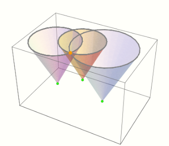
Essentially, the solution, [math]\displaystyle{ \scriptstyle (\hat{\boldsymbol{r}}_{\text{rec}},\, \hat{t}_{\text{rec}}) }[/math], is the intersection of light cones. https://handwiki.org/wiki/index.php?curid=2077021
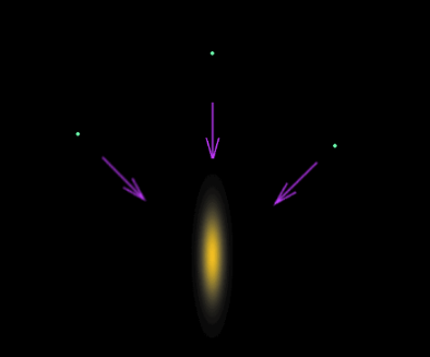
The posterior distribution of the solution is derived from the product of the distribution of propagating spherical surfaces. (See animation.). https://handwiki.org/wiki/index.php?curid=1327270
3. The GPS Case
- For Global Positioning System (GPS),[2] the non-closed-form equations in step 3 result in
- [math]\displaystyle{ \scriptstyle \begin{cases} \scriptstyle \Delta t_i (t_i,\, E_i) \;\triangleq\; t_i \,+\, \delta t_{\text{clock},i} (t_i,\, E_i) \,-\, \tilde{t}_i \;=\; 0, \\ \scriptstyle \Delta M_i (t_i,\, E_i) \;\triangleq\; M_i (t_i) \,-\, (E_i \,-\, e_i \sin E_i) \;=\; 0, \end{cases} }[/math]
in which [math]\displaystyle{ \scriptstyle E_i }[/math] is the orbital eccentric anomaly of satellite [math]\displaystyle{ i }[/math], [math]\displaystyle{ \scriptstyle M_i }[/math] is the mean anomaly, [math]\displaystyle{ \scriptstyle e_i }[/math] is the eccentricity, and [math]\displaystyle{ \scriptstyle \delta t_{\text{clock},i} (t_i,\, E_i) \;=\; \delta t_{\text{clock,sv},i} (t_i) \,+\, \delta t_{\text{orbit-relativ},i} (E_i) }[/math].
- The above can be solved by using the bivariate Newton–Raphson method on [math]\displaystyle{ \scriptstyle t_i }[/math] and [math]\displaystyle{ \scriptstyle E_i }[/math]. Two times of iteration will be necessary and sufficient in most cases. Its iterative update will be described by using the approximated inverse of Jacobian matrix as follows:
[math]\displaystyle{ \scriptstyle \begin{pmatrix} t_i \\ E_i \\ \end{pmatrix} \leftarrow \begin{pmatrix} t_i \\ E_i \\ \end{pmatrix} - \begin{pmatrix} 1 && 0 \\ \frac{\dot{M}_i (t_i)}{1 - e_i \cos E_i} && -\frac{1}{1 - e_i \cos E_i} \\ \end{pmatrix} \begin{pmatrix} \Delta t_i \\ \Delta M_i \\ \end{pmatrix} }[/math]
- Tropospheric delay should not be ignored, while the Global Positioning System (GPS) specification[2] doesn't provide its detailed description.
4. The GLONASS Case
- The GLONASS ephemerides don't provide clock biases [math]\displaystyle{ \scriptstyle\delta t_{\text{clock,sv},i} (t) }[/math], but [math]\displaystyle{ \scriptstyle\delta t_{\text{clock},i} (t) }[/math].
References
- Misra, P. and Enge, P., Global Positioning System: Signals, Measurements, and Performance, 2nd, Ganga-Jamuna Press, 2006.
- The interface specification of NAVSTAR GLOBAL POSITIONING SYSTEM http://www.navcen.uscg.gov/pdf/IS-GPS-200D.pdf
- 3-dimensional distance is given by [math]\displaystyle{ \displaystyle r(\boldsymbol_A,\, \boldsymbol_B) = |\boldsymbol_A - \boldsymbol_B| = \sqrt{(x_A-x_B)^2+(y_A-y_B)^2+(z_A-z_B)^2} }[/math] where [math]\displaystyle{ \displaystyle\boldsymbol_A = (x_A, y_A, z_A) }[/math] and [math]\displaystyle{ \displaystyle\boldsymbol_B = (x_B, y_B, z_B) }[/math] represented in inertial frame.