Video Upload Options

1. Definitions of Stress Measures

Consider the situation shown in the following figure. The following definitions use the notations shown in the figure.

Quantities used in the definition of stress measures

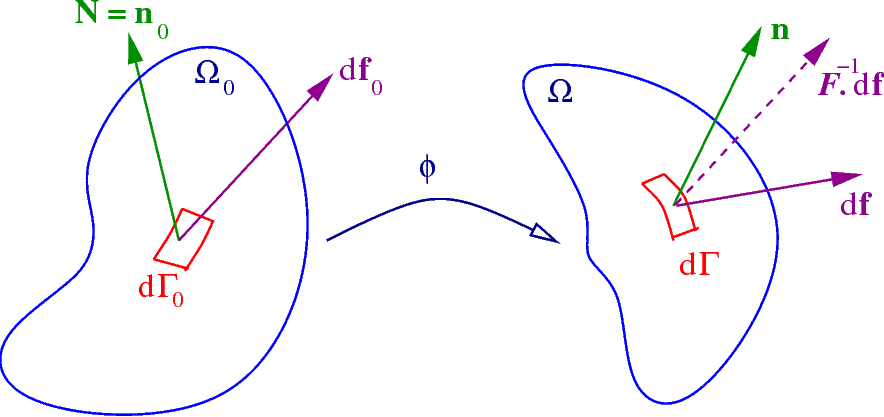In the reference configuration [math]\displaystyle{ \Omega_0 }[/math], the outward normal to a surface element [math]\displaystyle{ d\Gamma_0 }[/math] is [math]\displaystyle{ \mathbf{N} \equiv \mathbf{n}_0 }[/math] and the traction acting on that surface is [math]\displaystyle{ \mathbf{t}_0 }[/math] leading to a force vector [math]\displaystyle{ d\mathbf{f}_0 }[/math]. In the deformed configuration [math]\displaystyle{ \Omega }[/math], the surface element changes to [math]\displaystyle{ d\Gamma }[/math] with outward normal [math]\displaystyle{ \mathbf{n} }[/math] and traction vector [math]\displaystyle{ \mathbf{t} }[/math] leading to a force [math]\displaystyle{ d\mathbf{f} }[/math]. Note that this surface can either be a hypothetical cut inside the body or an actual surface. The quantity [math]\displaystyle{ \boldsymbol{F} }[/math] is the deformation gradient tensor, [math]\displaystyle{ J }[/math] is its determinant.

1.1. Cauchy Stress

The Cauchy stress (or true stress) is a measure of the force acting on an element of area in the deformed configuration. This tensor is symmetric and is defined via

[math]\displaystyle{ d\mathbf{f} = \mathbf{t}~d\Gamma = \boldsymbol{\sigma}^T\cdot\mathbf{n}~d\Gamma }[/math]

or

[math]\displaystyle{ \mathbf{t} = \boldsymbol{\sigma}^T\cdot\mathbf{n} }[/math]

where [math]\displaystyle{ \mathbf{t} }[/math] is the traction and [math]\displaystyle{ \mathbf{n} }[/math] is the normal to the surface on which the traction acts.

1.2. Kirchhoff Stress

The quantity,

[math]\displaystyle{ \boldsymbol{\tau} = J~\boldsymbol{\sigma} }[/math]

is called the Kirchhoff stress tensor, with [math]\displaystyle{ J }[/math] the determinant of [math]\displaystyle{ \boldsymbol{F} }[/math]. It is used widely in numerical algorithms in metal plasticity (where there is no change in volume during plastic deformation). It can be called weighted Cauchy stress tensor as well.

1.3. Nominal Stress/First Piola-Kirchhoff Stress

The nominal stress [math]\displaystyle{ \boldsymbol{N}=\boldsymbol{P}^T }[/math] is the transpose of the first Piola-Kirchhoff stress (PK1 stress, also called engineering stress) [math]\displaystyle{ \boldsymbol{P} }[/math] and is defined via

[math]\displaystyle{ d\mathbf{f} = \mathbf{t}~d\Gamma = \boldsymbol{N}^T\cdot\mathbf{n}_0~d\Gamma_0 = \boldsymbol{P}\cdot\mathbf{n}_0~d\Gamma_0 }[/math]

or

[math]\displaystyle{ \mathbf{t}_0 =\mathbf{t}\dfrac{d{\Gamma}}{d\Gamma_0}= \boldsymbol{N}^T\cdot\mathbf{n}_0 = \boldsymbol{P}\cdot\mathbf{n}_0 }[/math]

This stress is unsymmetric and is a two-point tensor like the deformation gradient.
The asymmetry derives from the fact that, as a tensor, it has one index attached to the reference configuration and one to the deformed configuration.^[1]

1.4. Second Piola-Kirchhoff Stress

If we pull back [math]\displaystyle{ d\mathbf{f} }[/math] to the reference configuration, we have

[math]\displaystyle{ d\mathbf{f}_0 = \boldsymbol{F}^{-1}\cdot d\mathbf{f} }[/math]

or,

[math]\displaystyle{ d\mathbf{f}_0 = \boldsymbol{F}^{-1}\cdot \boldsymbol{N}^T\cdot\mathbf{n}_0~d\Gamma_0 = \boldsymbol{F}^{-1}\cdot \mathbf{t}_0~d\Gamma_0 }[/math]

The PK2 stress ([math]\displaystyle{ \boldsymbol{S} }[/math]) is symmetric and is defined via the relation

[math]\displaystyle{ d\mathbf{f}_0 = \boldsymbol{S}^T\cdot\mathbf{n}_0~d\Gamma_0 = \boldsymbol{F}^{-1}\cdot \mathbf{t}_0~d\Gamma_0 }[/math]

Therefore,

[math]\displaystyle{ \boldsymbol{S}^T\cdot\mathbf{n}_0 = \boldsymbol{F}^{-1}\cdot\mathbf{t}_0 }[/math]

1.5. Biot Stress

The Biot stress is useful because it is energy conjugate to the right stretch tensor [math]\displaystyle{ \boldsymbol{U} }[/math]. The Biot stress is defined as the symmetric part of the tensor [math]\displaystyle{ \boldsymbol{P}^T\cdot\boldsymbol{R} }[/math] where [math]\displaystyle{ \boldsymbol{R} }[/math] is the rotation tensor obtained from a polar decomposition of the deformation gradient. Therefore, the Biot stress tensor is defined as

[math]\displaystyle{ \boldsymbol{T} = \tfrac{1}{2}(\boldsymbol{R}^T\cdot\boldsymbol{P} + \boldsymbol{P}^T\cdot\boldsymbol{R}) ~. }[/math]

The Biot stress is also called the Jaumann stress.

The quantity [math]\displaystyle{ \boldsymbol{T} }[/math] does not have any physical interpretation. However, the unsymmetrized Biot stress has the interpretation

[math]\displaystyle{ \boldsymbol{R}^T~d\mathbf{f} = (\boldsymbol{P}^T\cdot\boldsymbol{R})^T\cdot\mathbf{n}_0~d\Gamma_0 }[/math]

2. Relations Between Stress Measures

2.1. Relations between Cauchy Stress and Nominal Stress

From Nanson's formula relating areas in the reference and deformed configurations:

[math]\displaystyle{ \mathbf{n}~d\Gamma = J~\boldsymbol{F}^{-T}\cdot\mathbf{n}_0~d\Gamma_0 }[/math]

Now,

[math]\displaystyle{ \boldsymbol{\sigma}^T\cdot\mathbf{n}~d\Gamma = d\mathbf{f} = \boldsymbol{N}^T\cdot\mathbf{n}_0~d\Gamma_0 }[/math]

Hence,

[math]\displaystyle{ \boldsymbol{\sigma}^T\cdot (J~\boldsymbol{F}^{-T}\cdot\mathbf{n}_0~d\Gamma_0) = \boldsymbol{N}^T\cdot\mathbf{n}_0~d\Gamma_0 }[/math]

or,

[math]\displaystyle{ \boldsymbol{N}^T = J~(\boldsymbol{F}^{-1}\cdot\boldsymbol{\sigma})^T = J~\boldsymbol{\sigma}^T\cdot\boldsymbol{F}^{-T} }[/math]

or,

[math]\displaystyle{ \boldsymbol{N} = J~\boldsymbol{F}^{-1}\cdot\boldsymbol{\sigma} \qquad \text{and} \qquad \boldsymbol{N}^T = \boldsymbol{P} = J~\boldsymbol{\sigma}^T\cdot\boldsymbol{F}^{-T} }[/math]

In index notation,

[math]\displaystyle{ N_{Ij} = J~F_{Ik}^{-1}~\sigma_{kj} \qquad \text{and} \qquad P_{iJ} = J~\sigma_{ki}~F^{-1}_{Jk} }[/math]

Therefore,

[math]\displaystyle{ J~\boldsymbol{\sigma} = \boldsymbol{F}\cdot\boldsymbol{N} = \boldsymbol{F}\cdot\boldsymbol{P}^T~. }[/math]

Note that [math]\displaystyle{ \boldsymbol{N} }[/math] and [math]\displaystyle{ \boldsymbol{P} }[/math] are (generally) not symmetric because [math]\displaystyle{ \boldsymbol{F} }[/math] is (generally) not symmetric.

2.2. Relations between Nominal Stress and Second P-K Stress

Recall that

[math]\displaystyle{ \boldsymbol{N}^T\cdot\mathbf{n}_0~d\Gamma_0 = d\mathbf{f} }[/math]

and

[math]\displaystyle{ d\mathbf{f} = \boldsymbol{F}\cdot d\mathbf{f}_0 = \boldsymbol{F} \cdot (\boldsymbol{S}^T \cdot \mathbf{n}_0~d\Gamma_0) }[/math]

Therefore,

[math]\displaystyle{ \boldsymbol{N}^T\cdot\mathbf{n}_0 = \boldsymbol{F}\cdot\boldsymbol{S}^T\cdot\mathbf{n}_0 }[/math]

or (using the symmetry of [math]\displaystyle{ \boldsymbol{S} }[/math]),

[math]\displaystyle{ \boldsymbol{N} = \boldsymbol{S}\cdot\boldsymbol{F}^T \qquad \text{and} \qquad \boldsymbol{P} = \boldsymbol{F}\cdot\boldsymbol{S} }[/math]

In index notation,

[math]\displaystyle{ N_{Ij} = S_{IK}~F^T_{jK} \qquad \text{and} \qquad P_{iJ} = F_{iK}~S_{KJ} }[/math]

Alternatively, we can write

[math]\displaystyle{ \boldsymbol{S} = \boldsymbol{N}\cdot\boldsymbol{F}^{-T} \qquad \text{and} \qquad \boldsymbol{S} = \boldsymbol{F}^{-1}\cdot\boldsymbol{P} }[/math]

2.3. Relations between Cauchy Stress and Second P-K Stress

Recall that

[math]\displaystyle{ \boldsymbol{N} = J~\boldsymbol{F}^{-1}\cdot\boldsymbol{\sigma} }[/math]

In terms of the 2nd PK stress, we have

[math]\displaystyle{ \boldsymbol{S}\cdot\boldsymbol{F}^T = J~\boldsymbol{F}^{-1}\cdot\boldsymbol{\sigma} }[/math]

Therefore,

[math]\displaystyle{ \boldsymbol{S} = J~\boldsymbol{F}^{-1}\cdot\boldsymbol{\sigma}\cdot\boldsymbol{F}^{-T} = \boldsymbol{F}^{-1}\cdot\boldsymbol{\tau}\cdot\boldsymbol{F}^{-T} }[/math]

In index notation,

[math]\displaystyle{ S_{IJ} = F_{Ik}^{-1}~\tau_{kl}~F_{Jl}^{-1} }[/math]

Since the Cauchy stress (and hence the Kirchhoff stress) is symmetric, the 2nd PK stress is also symmetric.

Alternatively, we can write

[math]\displaystyle{ \boldsymbol{\sigma} = J^{-1}~\boldsymbol{F}\cdot\boldsymbol{S}\cdot\boldsymbol{F}^T }[/math]

or,

[math]\displaystyle{ \boldsymbol{\tau} = \boldsymbol{F}\cdot\boldsymbol{S}\cdot\boldsymbol{F}^T ~. }[/math]

Clearly, from definition of the push-forward and pull-back operations, we have

[math]\displaystyle{ \boldsymbol{S} = \varphi^{*}[\boldsymbol{\tau}] = \boldsymbol{F}^{-1}\cdot\boldsymbol{\tau}\cdot\boldsymbol{F}^{-T} }[/math]

and

[math]\displaystyle{ \boldsymbol{\tau} = \varphi_{*}[\boldsymbol{S}] = \boldsymbol{F}\cdot\boldsymbol{S}\cdot\boldsymbol{F}^T~. }[/math]

Therefore, [math]\displaystyle{ \boldsymbol{S} }[/math] is the pull back of [math]\displaystyle{ \boldsymbol{\tau} }[/math] by [math]\displaystyle{ \boldsymbol{F} }[/math] and [math]\displaystyle{ \boldsymbol{\tau} }[/math] is the push forward of [math]\displaystyle{ \boldsymbol{S} }[/math].

References

- Three-Dimensional Elasticity. Elsevier. 1 April 1988. ISBN 978-0-08-087541-5. https://books.google.com/books?id=tlGCC3w27iIC.