 +1 credit
| Version | Summary | Created by | Modification | Content Size | Created at | Operation |
|---|---|---|---|---|---|---|
| 1 | Sirius Huang | -- | 1524 | 2022-11-04 01:42:22 |
Video Upload Options
An equitable division (EQ) is a division of a heterogeneous object (e.g. a cake), in which the subjective value of all partners is the same, i.e., each partner is equally happy with his/her share.
1. Comparison to Other Criteria
- Equitability (EQ) compares values of different people to different pieces;
- Envy-freeness (EF) compares values of the same person to different pieces;
- Exact division (EX) compares values of different people to the same pieces.
The following table illustrates the difference. In all examples there are two partners, Alice and Bob. Alice receives the left part and Bob receives the right part.
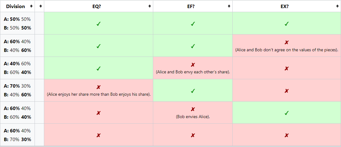
Note that the table has only 6 rows, because 2 combinations are impossible: an EX+EF division must be EQ, and an EX+EQ division must be EF.
2. Finding an Equitable Division for Two Partners
2.1. One Cut - Full Revelation
When there are 2 partners, it is possible to get an EQ division with a single cut, but it requires full knowledge of the partners' valuations.[1] Assume that the cake is the interval [0,1]. For each [math]\displaystyle{ x\in[0,1] }[/math], calculate [math]\displaystyle{ u_1([0,x]) }[/math] and [math]\displaystyle{ u_2([x,1]) }[/math] and plot them on the same graph. Note that the first graph is increasing from 0 to 1 and the second graph is decreasing from 1 to 0, so they have an intersection point. Cutting the cake at that point yields an equitable division. This division has several additional properties:
- It is EF, since each partner receives a value of at least 1/2.
- It is not EX, since the value per partner may be more than 1/2.
- It is Pareto efficient (PE) among all divisions that use a single cut. However, there may be more efficient divisions that use two or more cuts.[2]
- If the direction of the cake is chosen at random (i.e. it can be flipped such that 0 becomes 1 and 1 becomes 0), then this procedure is also weakly truthful, in the following sense: only by submitting sincere probability measures, can a partner ensure that he receives at least half of the cake.[1]
The same procedure can be used for dividing chores (with negative utility).
Proportional-equitability variant
The full revelation procedure has a variant[3] which satisfies a weaker kind of equitability and a stronger kind of truthfulness. The procedure first finds the median points of each partner. Suppose the median point of partner A is [math]\displaystyle{ a }[/math] and of partner B is [math]\displaystyle{ b }[/math], with [math]\displaystyle{ 0\lt a\lt b\lt 1 }[/math]. Then, A receives [math]\displaystyle{ [0,a] }[/math] and B receives [math]\displaystyle{ [b,1] }[/math]. Now there is a surplus - [math]\displaystyle{ [a,b] }[/math]. The surplus is divided between the partners in equal proportions. So, for example, if A values the surplus as 0.4 and B values the surplus as 0.2, then A will receive twice more value from [math]\displaystyle{ [a,b] }[/math] than B. So this protocol is not equitable, but it is still EF. It is weakly-truthful in the following sense: a risk-averse player has an incentive to report his true valuation, because reporting an untrue valuation might leave him with a smaller value.
2.2. Two Cuts - Moving Knife
Austin moving-knife procedure gives each of the two partners a piece with a subjective value of exactly 1/2. Thus the division is EQ, EX and EF. It requires 2 cuts, and gives one of the partners two disconnected pieces.
2.3. Many Cuts - Full Revelation
When more than two cuts are allowed, it is possible to achieve a division which is not only EQ but also EF and PE. Some authors call such a division "perfect".[4]
The minimum number of cuts required for a PE-EF-EQ division depends on the valuations of the partners. In most practical cases (including all cases when the valuations are piecewise-linear) the number of required cuts is finite. In these cases, it is possible to both find the optimal number of cuts and their exact locations. The algorithm requires full knowledge of the partners' valuations.[4]
2.4. Run-Time
All the above procedures are continuous: the second requires a knife that moves continuously, the others requires a continuous plot of the two value measures. Therefore, they cannot be carried out in a finite number of discrete steps.
This infinity property is characteristic of division problems which require an exact result. See Exact division.
2.5. One Cut - Near-Equitable Division
A near-equitable division is a division in which the partners' values differ by at most [math]\displaystyle{ \epsilon }[/math], for any given [math]\displaystyle{ \epsilon\gt 0 }[/math]. A near-equitable division for two partners can be found in finite time and with a single cut.[5]
3. Finding an Equitable Division for Three or More Partners
3.1. Moving Knife Procedure
Austin's procedure can be extended to n partners. It gives each partner a piece with a subjective value of exactly [math]\displaystyle{ 1/n }[/math]. This division is EQ, but not necessarily EX or EF or PE (since some partners may value the share given to other partners as more than [math]\displaystyle{ 1/n }[/math]).
3.2. Connected Pieces - Full Revelation
Jones' full revelation procedure can be extended to [math]\displaystyle{ n }[/math] partners in the following way:[3]
- For each of the [math]\displaystyle{ n! }[/math] possible orderings of the partners, write a set of [math]\displaystyle{ n-1 }[/math] equations in [math]\displaystyle{ n-1 }[/math] variables: the variables are the [math]\displaystyle{ n-1 }[/math] cut-points, and the equations determine the equitability for adjacent partners. For example, of there are 3 partners and the order is A:B:C, then the two variables are [math]\displaystyle{ x_{AB} }[/math] (the cut-point between A and B) and [math]\displaystyle{ x_{BC} }[/math], and the two equations are [math]\displaystyle{ V_A(0,x_{AB})=V_B(x_{AB},x_{BC}) }[/math] and [math]\displaystyle{ V_B(x_{AB},x_{BC})=V_C(x_{BC},1) }[/math]. These equations have at least one solution in which all partners have the same value.
- Out of all [math]\displaystyle{ n! }[/math] orderings, pick the ordering in which the (equal) value of all partners is the largest.
Note that the maximal equitable value must be at least [math]\displaystyle{ 1/n }[/math], because we already know that a proportional division (giving each partner at least [math]\displaystyle{ 1/n }[/math]) is possible.
If the value measures of the partners are absolutely continuous with respect to each other (this means that they have the same support), then any attempt to increase the value of a partner must decrease the value of another partner. This means that the solution is PE among the solutions which give connected pieces.
3.3. Impossibility Results
Brams, Jones and Klamler study a division which is EQ, PE and EF (they call such a division "perfect").
They first prove that, for 3 partners that must get connected pieces, an EQ+EF division may not exist.[3] They do this by describing 3 specific value measures on a 1-dimensional cake, in which every EQ allocation with 2 cuts is not EF.
Then they prove that, for 3 or more partners, a PE+EF+EQ division may not exist even with disconnected pieces.[2] They do this by describing 3 specific value measures on a 1-dimensional cake, with the following properties:
- With 2 cuts, every EQ allocation is not EF nor PE (but there are allocations which are EF and 2-PE, or EQ and 2-PE).
- With 3 cuts, every EQ allocation is not PE (but there is an EQ+EF allocation).
- With 4 cuts, every EQ allocation is not EF (but there is an EQ+PE allocation).
3.4. Pie Cutting
A pie is a cake in the shape of a 1-dimensional circle (see fair pie-cutting).
Barbanel, Brams and Stromquist study the existence of divisions of a pie, which are both EQ and EF. The following existence results are proved without providing a specific division algorithm:[6]
- For 2 partners, there always exists a partition of a pie which is both envy-free and equitable. When the value measures of the partners are absolutely continuous with respect to each other (i.e. every piece which has a positive value for one partner also has a positive value for the other partner), then there exists a partition which is envy-free, equitable and undominated.
- For 3 or more partners, it may be impossible to find an allocation that is both envy-free and equitable. But there always exists a division that is both equitable and undominated.
3.5. Divisible Goods
The adjusted winner procedure calculates an equitable, envy-free and efficient division of a set of divisible goods between two partners.
4. Query Complexity
An equitable cake allocation cannot be found using a finite protoocl in the Robertson–Webb query model, even for 2 agents.[7] Moreover, for any ε > 0:
- A connected ε-equitable cake-cutting requires at least Ω(log ε−1) queries.[8] For 2 agents, an O(log ε−1) protocol exists.[5] For 3 or more agents, the best known protocol requires O(n (log n + log ε−1)) queries.[9]
- Even without connectivity, ε-equitable cake-cutting requires at least Ω(log ε−1 / log log ε−1 ) queries.[7]
5. Summary Table
| Name | Type | # partners | # cuts | Properties |
|---|---|---|---|---|
| Jones[1] | Full-revelation proc | 2 | 1 (optimal) | EQ, EF, 1-PE |
| Brams-Jones-Klamler[3] | Full-revelation proc | n | n−1 (optimal) | EQ, (n−1)-PE |
| Austin | Moving-knife proc | 2 | 2 | EQ, EF, EX |
| Austin | Moving-knife proc | n | many | EQ |
| Barbanel-Brams[4] | Full-revelation proc | 2 | many | EQ, EF, PE |
| Cechlárová-Pillárová[5] | Discrete approximation proc | 2 | 1 (optimal) | near-EQ |
References
- Jones, M. A. (2002). "Equitable, Envy-Free, and Efficient Cake Cutting for Two People and Its Application to Divisible Goods". Mathematics Magazine 75 (4): 275–283. doi:10.2307/3219163. https://dx.doi.org/10.2307%2F3219163
- Steven j. Brams; Michael a. Jones; Christian Klamler (2013). "N-Person Cake-Cutting: There May Be No Perfect Division". The American Mathematical Monthly 120: 35. doi:10.4169/amer.math.monthly.120.01.035. https://dx.doi.org/10.4169%2Famer.math.monthly.120.01.035
- Steven J. Brams; Michael A. Jones; Christian Klamler (2007). "Better Ways to Cut a Cake - Revisited". Notices of the AMS. http://vesta.informatik.rwth-aachen.de/opus/volltexte/2007/1227/pdf/07261.KlamlerChristian.Paper.1227.pdf.
- Barbanel, Julius B.; Brams, Steven J. (2014). "Two-Person Cake Cutting: The Optimal Number of Cuts". The Mathematical Intelligencer 36 (3): 23. doi:10.1007/s00283-013-9442-0. https://dx.doi.org/10.1007%2Fs00283-013-9442-0
- Cechlárová, Katarína; Pillárová, Eva (2012). "A near equitable 2-person cake cutting algorithm". Optimization 61 (11): 1321. doi:10.1080/02331934.2011.563306. https://dx.doi.org/10.1080%2F02331934.2011.563306
- Barbanel, J. B.; Brams, S. J.; Stromquist, W. (2009). "Cutting a Pie is Not a Piece of Cake". American Mathematical Monthly 116 (6): 496. doi:10.4169/193009709X470407. https://dx.doi.org/10.4169%2F193009709X470407
- Procaccia, Ariel D.; Wang, Junxing (2017-06-20). "A Lower Bound for Equitable Cake Cutting". Proceedings of the 2017 ACM Conference on Economics and Computation. EC '17 (Cambridge, Massachusetts, USA: Association for Computing Machinery): 479–495. doi:10.1145/3033274.3085107. ISBN 978-1-4503-4527-9. https://doi.org/10.1145/3033274.3085107.
- Brânzei, Simina; Nisan, Noam (2018-07-13). "The Query Complexity of Cake Cutting". arXiv:1705.02946 [cs.GT]. //arxiv.org/archive/cs.GT
- Cechlárová, Katarína; Pillárová, Eva (2012-11-01). "On the computability of equitable divisions" (in en). Discrete Optimization 9 (4): 249–257. doi:10.1016/j.disopt.2012.08.001. ISSN 1572-5286. https://www.sciencedirect.com/science/article/pii/S1572528612000606.

