Low Earth Orbit Space Missions Power Bus Management

Version	Summary	Created by	Modification	Content Size	Created at	Operation
1		Luigi Schirone	+ 2775 word(s)	2775	2021-11-30 05:31:49	\|
2	format correct	Conner Chen	Meta information modification	2775	2021-12-06 06:59:48	\|

This entry is adapted from the peer-reviewed paper 10.3390/en14237932

In space vehicles, the typical configurations for the Solar Array Power Regulators in charge of managing power transfer from the solar array to the power bus are quite different from the corresponding devices in use for terrestrial applications. Since the 1970s the most widely used approach for spacecraft power conditioning has been Sequential Switching Shunt Regulation (S3R), because of its high power density, modularity, simplicity, and inherently high reliability. Power regulation schemes implementing Maximum Power Point Tracking (MPPT) techniques have been introduced since the 1990s. At the expense of a larger complexity, they provide optimal energy harvesting in a wide range of operating conditions. In sectional MPPT power units, the solar array is split into several sections, each fitted up with a dedicated Solar Array Power Regulator (APR) with a multimode controller, capable of either independently performing MPPT or harmonically contributing to the regulation of the bus voltage or the battery current. An expedient solution appears to be provided by the Sequential Maximum Power Tracking (SMPT) bus regulation technique: the coordination problem is solved by implementing an operational sequence such that just one section at a time is kept in control mode, while the others are kept either in MPPT or in standby.

satellite power sources solar array regulation module battery charge/discharge regulation module maximum power point tracking (MPPT) SMPT

1. Comparison among the Regulation Techniques

A trade-off analysis of the considered regulation techniques has been developed. The analyses are in reference to a specific case study, an Earth Observation Spacecraft flying in a Sun-synchronous orbit at 380 km altitude, characterized by ^[1], an orbital period T0 = 90 min, with 30 min eclipse duration. This trend is typical for low Earth orbits: the exact value of the irradiance duty cycle depends on orbital altitude, inclination, and eccentricity, and in a circular orbit it is lightly larger than 66% at 300 km, and smaller than 60% at 1500 km. Only in very special orbits it can be close to 100% (e.g., in down-dusk orbits, where the orbital plane is almost orthogonal to the solar vector). Due to this variability, we were forced to develop our analyses in reference to a very specific space mission, assuming that the general conclusions could be extended to similar applications, including many low Earth orbits with pulsed loads.

In order to perform a straight trade-off analysis, the solar radiation collected by the panels has been assumed to be only affected by eclipses (step transitions from darkness to sunlight, neglecting penumbra times) and by solar panel temperature. As the actual solar cell temperature depends on the details of the solar panels, in our analyses we referred to typical textbook data for low Earth orbit missions ^[2] (Sections 9.3–4) and assumed that temperature was in the range −60 °C (at the end of eclipse) to +40 °C (at the beginning of eclipse). Figure 1 reports the trends considered for this trade-off analysis for irradiation (orange curve, right axis) and temperature (blue curve, left axis).

Figure 1. Irradiation (orange curve, right axis) and solar cell temperature (blue curve, left axis) in the considered orbit.

The solar array considered for this case study was able to provide 1.4 kW in AM0 at Beginning of Life and consisted of 1088 triple-junction solar cells, model CTJ30 by CESI, arranged in 64 strings of 17 series-connected cells, grouped as 8 independent sections. The analyses were based on their expected performance after aging by absorption of a radiation fluence of 5 × 10¹⁴ equivalent 1 MeV electrons, corresponding to several years in a typical Sun-synchronous polar orbit.

In order to stress differences among the regulation approaches investigated in this work, mismatching among solar array sections has been taken into account. In particular, it was assumed that a section underwent a relevant reduction of the output voltage, which in real operation may be caused by damaging or shadowing a group of solar cells, with activation of the dedicated bypass diodes.

Table 1 collects the values of Open Circuit Voltage (V_OC), Short Circuit Current (I_SC) and their thermal coefficients considered for the different solar array sections.

Table 1. Electrical parameters of the solar array sections.

Sec. 1–5	Sec. 6	Sec. 7	Sec. 8
V_OC (V) @AM0	41.8	44.4	39.2	31.3
I_SC (A) @AM0	4.2	4.1	4.3	4.2
ΔV_OC/ΔT (%/°C)	−0.217	−0.217	−0.217	−0.217
ΔI_SC/ΔT (%/°C)	+0.0964	+0.0964	+0.0964	+0.0964

The model for Solar Arrays accounts for temperature effects on the solar cell characteristics. Based on the thermal coefficients and other specification data published by the manufacturers ^[3], estimated current–voltage pairs for a representative set of temperatures were collected in a Look-Up-Table, allowing derivation by interpolating the current–voltage characteristics at any temperature in the considered range.

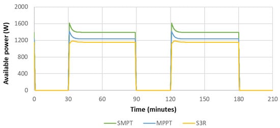
The available power depends on the regulation approach, as reported in Figure 2. When the loads absorb all available power from the solar array, in S³R all sections in parallel are tied to the bus voltage; in MPPT all sections in parallel are kept at the voltage corresponding to the maximum power point of the overall solar array; in SMPT optimal energy harvesting is achieved as each section independently is kept at the voltage corresponding to its Maximum Power Point.

Figure 2. Available power from the solar array with the different regulation approaches.

The difference between the curves related to SMPT and MPPT is related to mismatching in the solar array: the common node in basic MPPT regulators keeps some sections at a voltage different from their actual V_MP, whereas in the sectional MPPT approaches, such as SMPT regulation, all solar array sections are working at their optimal voltage. Otherwise, in S³R the operating voltage for solar arrays is fixed independently of the variations of V_MP. Furthermore, due to the negative thermal coefficient for voltages, after some minutes in sunlight the sections starting with the smaller V_OC may be forced to work in the low-current region of their characteristics, with appreciable power reductions. In Figure 3 it is clearly seen that this happens for the section 8 in the solar array, whose open-circuit voltage at 25 °C was just 3.3 V larger than the bus voltage.

Figure 3. With S³R all solar array sections but section 8 supply the same output power (section 8 has a relevant decrease in Voc, whereas minor differences among Voc of sections 1–7 exist, so that the curves are superimposed).

The load profile considered for the spacecraft is reported in Figure 4. Basic activities absorb 200 W both in sunlight and in eclipse, and periodically the operations of the payload or some spacecraft subsystems result in additional peaks of 900 W for 5 min and 3.2 kW for 1 min. The conversion efficiency was assumed to be 96% for S³R and 92% for both MPPT-APRs and SMPT-APRs.

Figure 4. The considered load waveforms.

The battery supplies the spacecraft during eclipses and load peaks. During sunlight it absorbs 200 W for recharging, whenever enough power for the purpose is available (see Figure 5, lower curves, left axis). During the peaks of load absorption, the battery stops charging and, when needed, sustains the load with suitable discharge pulses.

Figure 5. Battery State of Charge (upper curves, right axis) and Charging Power for battery (lower curves, left axis).

The trend of the battery State of Charge (SoC) (Figure 9, upper curves, right axis) shows that high load pulses may result in deep cycles in the battery: as expected, the depth of discharge is at a maximum for S³R. This could affect battery duration ^[2] and shall be compensated by increasing the size of the battery.

For the considered case study, the overall amounts of energy per orbit delivered by MPPT and S³R are quite similar, as the larger efficiency of S³R is compensated by the poorer harvesting of the power available on the solar array. For the chosen solar array, the MPPT regulator completes battery recharging with a small margin with respect to the available sunlight time, whereas the S³R regulator is not able to fully recharge the battery recharging: larger solar arrays would be needed to enable energy balance with S³R.

Otherwise, the larger amount of available power, as shown in Figure 6, enables the SMPT regulator to complete battery recharging well in advance of the next eclipse. It is clear that the case study was specifically built to highlight the strengths of the sectional MPPT approaches such as SMPT, but there is no doubt that these regulation techniques provide clear-cut advantages in terms of performance.

2. SMPT Simulation and Experimental Results

A model of the SMPT regulator was developed in Simulink, aiming to demonstrate the operation of the sequencing algorithm. As shown in Figure 6, the system consists of four blocks, each comprising a solar array section (in blue), an APR consisting of a dc–dc converter (in grey), and a dedicated controller in charge of managing the SMPT sequence on the basis of the status signals coming from other blocks as well as regulating the APR output current (Iout) to enforce the desired overall control law for the battery and the power bus. All converter outputs are connected in parallel and supply a battery and a variable resistive load.

Figure 6. Simulink model of the SMPT technique. The subsystem blocks (in grey) model the SEPIC converters directly from their circuit schematics. The blue blocks are library blocks for photovoltaic arrays.

The converter configuration is SEPIC ^[4], providing both step-up and step-down operation to allow the solar array sections to operate at voltages across the battery voltage. The circuit embedded in the submodel blocks is reported in Figure 7.

Figure 7. Submodel block for the SEPIC converters.

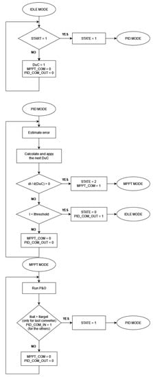
The control block of any APR sets the operating mode according to the observed battery current, to the Duty Cycle (DuC) of the corresponding converter and to the status signals received from other APRs (see Figure 8). Any single controller can work in three different modes:

Figure 8. Flow chart of the control algorithm.

State 0: the converter is in IDLE mode, and the controller applies a default Duty Cycle (DuC) of 1, forcing the output of the photovoltaic source in short-circuit. This solution was preferred to the option of getting the idle mode with the source in open-circuit because it allows easier management of the end of eclipses.
State 1: the controller runs the PID algorithm for control, modulating the converter DuC to stabilize the battery charging current.
State 2: the controller is the MPPT mode, running a basic Perturb and Observe (P&O) algorithm, intended to maximize the contribution from the single block, while another APR in the sequence is in charge of fine control.

Changes of state are triggered by the signals shared with the other APRs, namely two signal lines shared with the previous APR in the start-up sequence and one signal line with the next one. More precisely, they are:

the “START” signal. When received in input, forces an APR to exit IDLE mode and start PID control.
the “MPPT_COM” signal, asserted when the APR is in MPPT mode. It sets the START input of the next APR to 1.
the “PID_COM” signal, asserted when the output current of the APR drops below a specified threshold, leading the APR to enter in the IDLE mode. It forces the previous APR in the start-up sequence to stop the MPPT mode and to start the PID control.

In the Simulink model reported in Figure 6, the PID_COM_IN input and the MPPT_COM output are not provided in the last converter because there is no next converter, while the PID_COM_OUT is not provided in the first converter because there is no previous converter.

Operation is described in detail in the flow chart reported in Figure 8. An APR enters the PID control mode when it receives a positive level on the START input line. The operating mode passes to MPPT when a Maximum Power Point is detected via a change in the slope of the power-vs-duty cycle trend. At that moment, a START signal is sent to the next APR in the sequence, that enters the PID mode. Otherwise, in case the controller drives the APR output current to zero, the operating mode passes to IDLE and a signal on the PID_COM line forces the previous APR to exit MPPT and start PID mode. Adequate thresholds and hysteresis have been introduced to achieve smooth operation.

The simulation was carried out with the following parameters:

single-section maximum power: 125 W;
Battery start voltage: 26 V;
Nominal charging current: 4 A;
Battery capacity: 1 kWh;
Load sequence (see Figure 9): 400 W to 800 W to 400 W to 140 W (1.7 Ω to 0.85 Ω to 1.7 Ω to 4.8 Ω);
Discrete, step size 10⁻⁷ s.

Figure 9. Load profile for the simulation.

The system was turned on with the bus absorption at 400 W including the load, and with the charging current for the battery set to 4 A. As depicted in Figure 10, a first APR, say APR₁, is activated and its output current increases attempting to achieve power balance. After a few tens of milliseconds, its output current reaches its maximum and the APR₁ starts operating in MPPT while the next section is activated in regulation mode. The step is repeated for the solar array sections 2 and 3 until around 0.3 s. The power balance is achieved with APR₄ in regulation mode.

Figure 10. Waveforms provided by the Simulink model of the SMPT technique: Ibat: battery current; Iload: load current; Ioutn with n = 1 to 4: output current of APRn. All currents are in amperes.

After 0.75 s the load absorption is further increased to 800 W. When APR₄ also goes into MPPT, all the available power from the solar array is delivered to the load and the battery starts discharging at nearly 12 A to balance the load demand. The load absorption returns to 400 W at 1.8 s and the previous operating point is quickly recovered. At 2.5 s a further load variation reduces the load absorption to 140 W, and the solar array sections 4 and 3 sequentially quench their outputs. The final equilibrium is found with section 2 in the regulation mode. During the transients, the control on battery current loosens and some deviations with respect to the expected trend are observed. They are particularly evident at 0.75 s, 2.5 s, and 2.7 s. An improved design of the control law will reduce this effect.

The operation of the SMPT algorithm was also experimentally demonstrated by a PCDU breadboard based on SEPIC APR converters. The regulation controller and the SMPT sequencer were both embedded in automotive microcontrollers. A detailed description of the breadboard is out of the scope of this work.

The test setup is shown in Figure 11. The photovoltaic source was provided by a Keysight E4360 two-channel Solar Array Simulator, with both channels configured as V_OC = 44 V, I_SC = 3.3 A, V_MP = 39.5 V, and I_MP = 3.2 A in order to reproduce the typical current–voltage characteristics of solar array sections consisting of 102 triple-junction solar cells in AM0 conditions ^[3], arranged as 6 parallel strings of 17 solar cells in series. The output bus was directly connected to a storage unit consisting of a battery bank with 36 Li-ion cells (size 26650), arranged as 4 parallel strings of 9 cells (4P9S). At the beginning of the tests, the battery was at a voltage V_BAT = 30 V. During the tests, the load was provided by a Hewlett Packard 6060B electronic load, and the overall bus absorption was varied in the range 0–180 W in current-control mode, with the current for battery charging stabilized at 2 A.

Figure 11. The test setup (left): the breadboard PCDU is supplied by a Keysight E4360 Solar Array Simulator and drives a power bus connected to a 4P9S Li-ion battery and to the loads. The converter board of the PCDU (right), designed to accommodate up to eight channels.

The solar array voltages observed during the tests are shown in Figure 12. As it is possible to see, the controllers used short-circuit as a starting condition so that the operating point moved in the V < V_MP region, where the current is almost a constant. Therefore, the reported solar array voltage waveforms provide a glance at the input power of the different APRs.

Figure 12. Solar array voltages during a load peak. At turn-ON the operating point is controlled by the APR₁ (yellow trace) with the APR₂ (blue trace) at a base power level. When a load peak forces APR₁ into MPPT, APR₂ takes control of the operating point. The reverse transient for a load reduction also is shown.

At system turn-ON (t₁), the overall output power was P_OUT < 120 W, resulting from battery charging at 2 A, and an additional 60 W load in parallel. The APR₁ (yellow trace) was controlling the charging current, while APR₂ (blue trace) was set to a base condition, with output power smaller than 20 W, just to keep the converter in Continuous Conduction Mode. At t₂ the load was increased to 120 W (overall output power Pout = 180 W), the APR₁ was forced into MPPT, and the control passed to APR₂ (blue trace). Then, at t₃, the load returned to 60 W: APR₁ first kept the MPPT mode until the output power of APR₂ went below base power level (at t₄), then APR₁ started again to operate in the control mode. In the meantime, APR₂ was set again to 20 W. The waveforms also show the system turn-off at t₅.

References

Pisacane, V.L. Fundamentals of Space Systems, 2nd ed.; Oxford University Press Inc.: New York, NY, USA, 2005.
Patel, M.R. Spacecraft Power Systems, 1st ed.; CRC Press: Boca Raton, FL, USA, 2004.
Space Solar Cells—CESI. Available online: https://www.cesi.it/space-solar-cells/ (accessed on 21 June 2021).
Massey, R.P.; Snyder, E. High voltage single ended dc-dc converter. In Proceedings of the 1977 IEEE Power Electronics Specialists Conference, Palo Alto, CA, USA, 14–16 June 1977; pp. 156–159.

© Text is available under the terms and conditions of the Creative Commons Attribution (CC BY) license; additional terms may apply. By using this site, you agree to the Terms and Conditions and Privacy Policy.

Upload a video for this entry

Information

Subjects: Engineering, Aerospace

Contributor MDPI registered users' name will be linked to their SciProfiles pages. To register with us, please refer to https://encyclopedia.pub/register :

Luigi Schirone

View Times: 543

Update Date: 06 Dec 2021

Table of Contents

Video Upload Options

Confirm

1. Comparison among the Regulation Techniques

2. SMPT Simulation and Experimental Results

References