Natural Gas Consumption Model for Polish Industrial Consumers

Version	Summary	Created by	Modification	Content Size	Created at	Operation
1		Tomasz Chrulski	+ 2799 word(s)	2799	2021-11-25 02:07:32	\|
2	format correct	Bruce Ren	Meta information modification	2799	2021-12-06 01:58:36	\|

This entry is adapted from the peer-reviewed paper 10.3390/en14227649

The transmission of natural gas is a key element of the Polish energy system. The published data of the Polish distribution system operators and the transmission system operator on the volume of gaseous fuel transmitted indicate a growing trend in the consumption of energy produced from natural gas. In connection with the energy transformation, switching energy generation sources from hard coal to natural gas in Poland, it is important for transmission operators to know the future demand for gaseous fuel.

natural gas transmission system operator econometric model

1. Introduction

The motivation of the article was to present the cause–effect analysis of the influence of external factors on the consumption of natural gas by the Polish industry. The research was based on the most frequently used estimation method in economics, i.e., the least squares method. It is shown that by estimating the unknown model parameters with this method, it is possible to obtain estimates for which the model best provides a description of the observed data. In recent years there has been a lack of research on the proposed topic; the results of the analysis may be useful to illustrate the essence of this natural gas in the energy transition. The transmission of natural gas is one of the main components of the country’s energy system ^[1]. The published data of the operators of the national distribution system and the transmission system, regarding the volume of gaseous fuel transmitted, testify to an upward trend in the consumption of energy produced from natural gas ^[2]. The basic task of the operators transmitting natural gas to the final consumers is its safe delivery and the guarantee of the continuity of supplies without any disturbances, and ensuring the continuity of the supplies has a decisive impact on maintaining the energy security and maintaining stability of the economy based on natural gas sources ^[3].

In connection with energy transformation, the switch of energy production sources from hard coal to natural gas, it is crucial for transmission operators to predict the future demand for gaseous fuel ^[4]. Knowledge of future phenomena related to the consumption of gaseous fuel provides business decisions related to the possible expansion of the transmission system and thus in investing financial resources for this purpose. The prediction also provides quantitative information related to the interest in gaseous fuel among industrial consumers and checking the trend of natural gas consumption in Poland in the aspect of energy transition.

It should be emphasized in this context that the current energy transformation is significantly influenced by the European Union’s climate and energy policy, including its long-term vision of achieving climate neutrality by 2050. In reference to the European Union’s climate and energy policy, Poland has developed its energy policy until 2040. PEP2040 contributes to the implementation of the Paris Agreement concluded in December 2015 during the 21st Conference of the Parties to the United Nations Framework Convention on Climate Change (COP21) ^[5]. A critical element of PEP 2040 is natural gas, which is expected to be the bridge fuel in the energy transition. The national resource potential offers the possibility of independently covering the demand for coal and biomass, but most of the demand for natural gas has to be covered by imports.

Despite the increase in the number of recognized hydrocarbon fields (Table 1) from year to year, the volume of natural gas from national production transmitted to the national transmission system is decreasing (Figure 1). This confirms that diversification of supplies from various sources guarantees persistence security. The fossil energy resources (coal, oil, and natural gas) currently have no substitutes to match the required energy demand. Poland has no chance to be self-sufficient in covering the country’s demand for oil and natural gas ^[6]. Due to this fact, it is important to diversify the supply routes ^[7]. An important aspect of ensuring energy production in Poland is still the production of electricity from coal.

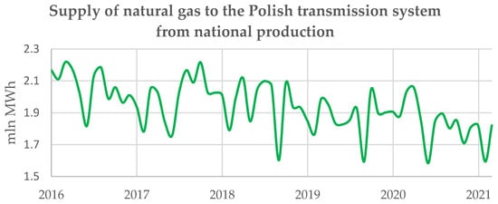
Figure 1. Supply of natural gas to the Polish transmission system from national production (2016–2021).

Table 1. Volume of recoverable natural gas reserves from gas, oil, and condensate fields in mln m3 (own elaboration based on data from Polish Geological Institute).

Year	Quantity of Reservoirs	Mines Resources	Off-Balance Reservoirs	Industrial Resources
2020	306	141,643.38	2277.13	73,514.38
2019	305	141,971.36	2277.67	74,953.67
2018	298	139,929.31	2230.59	66,640.98
2017	295	116,956.98	2230.26	50,607.8
2016	293	119,721.34	2219.85	52,295.1

Many factors may influence the consumption of natural gas by final consumers (industrial consumers, households) ^[8]. It is important to note that there is growing interest in gaseous fuel in Poland (Figure 2) Based on the literature on the subject, several potential factors can influence the consumption of natural gas in Poland and can be identified ^[9]^[10]. These are described in the following section. It is necessary to mention that the influence of the coronavirus pandemic on the volumes of transmitted natural gas volumes has also been noticed recently ^[11]. Consequently, there is no attempt to build a model for the years 2020–2021, as they are affected by the deformation of the time series related to the supply of gaseous fuels.

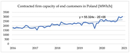
Figure 2. Supply of natural gas to Polish customers (2011–2015)

2. Natural Gas Consumption Model for Polish Industrial Consumers

Econometric modeling has shown that for the proposed macroeconomic indicators, the natural gas consumption by Polish industrial consumers is determined to the greatest extent by the heat and power industry and the chemical industry. A significant role is also played by increasing the contracting of firm capacity provided by the Polish gas transmission pipelines operator, which proves an increased interest in gaseous fuel by the industry. This interest is related to the ongoing transformation process, in which natural gas will constitute a bridge fuel and an important factor in ensuring energy security.

To build the model, historical data related to the supply of gaseous fuel were necessary. The analysis covered the years 2011–2021. In the analysed time interval, potential macroeconomic indicators and natural gas volumes shipped were given in monthly gradation. It was found that for the course of natural gas supply there are structural changes that make it necessary to analyse the time series in the periods January 2015–March 2018, March 2018–January 2020, and January 2020–December 2020 (COVID-19). The selected macroeconomic indicators confirmed the fact that structural changes occurred during the pandemic period. Therefore, a stable supply period was considered for the study, as required for the model, 2011–2015.

Initially, variables such as the share of Property Rights to Certificates of Origin for energy produced from RES (in order to present them as a new source in the ongoing energy transition) in session transactions on the Polish Power Exchange and hard coal production in Poland (energy transition process) were proposed. Other variables proposed are energy-related goods, construction and assembly production (constant prices), dwelling or house occupancy and energy carriers, price index of industrial output sold, weighted average gas prices.

Based on the information obtained from descriptive statistics, it was found that the coefficients of variation for the indicators: “coal production [thousand tonnes]”, “energy-related goods”, “dwelling or house use and energy carriers”, “price indices of industrial output sold” are low, that is, less than 0.1. For this reason, these indices were not taken into account for further analysis. In the article an attempt was made to present the dependence of the impact of energy produced from hard coal, but the low variability of the index did not allow it. Therefore, an additional variable was introduced, namely PCMSI 2 (Polish Energy Coal Market Index). Moreover, due to the fact that the above-mentioned indices could not be taken into account in further analysis, additional indices were carried out: the price of Brend crude oil, CO₂ emissions trading (EU ETS carbon market price euros), coefficients for the number of heating days, the coefficient for electricity/gas/steam/hot water generation and supply, new orders in the industry. An attempt was also made to introduce variables related to the length of available infrastructure and the number of new customers (connected and in the process of being connected), but without success due to lack of such data (protected data). For the above variables, the coefficients introduced were no longer low and were taken for further analysis. After analysing the time series graphs of the proposed variables, it was concluded that because of the too frequent structural changes occurring in the variable “coal production”, the elimination was eliminated.

Subsequently, a preliminary analysis of the graphs of the dependence of the explained variable (gas supply to end users) on the explanatory variables, as well as the dependence between the explanatory variables themselves, was carried out. The conclusions of the preliminary analysis showed that the explained variable is dependent.

From all variables, with the exception of the variable ‘price index of industrial production sold.’ Preliminary analysis revealed many unfavourable correlations between the explanatory variables.

Another important aspect was to assess the stationarity of the time series. The variables initially proposed can be used to build the model, but there is a risk of apparent regression. Therefore, the explanatory variable and the explained variables were tested for stationarity. The Dickey-Fuller test for the Y variable showed that it is a series with free expression, linear trend, and quadratic trend. The KPSS test confirmed this fact. The Dickey-Fuller and KPSS tests were used to check trend stability, stationarity, and stochastic nonstationarity for the remaining variables. The results obtained showed that the variables X1, X11, X12, and X13 are stationary. For the period 2016–2018, the series is stationary, it was noted that since the beginning of 2018 there has been a sharp increase for the variable X8, which causes a structural change and these observations were not taken into account.

After examining the series for stationarity, this was removed for the variables for which it was found. A preliminary analysis of the model was then carried out. The estimate of the model was carried out using the classical least-squares method. However, due to the very high p-value for the F-test (0.919), other variables that could be used in the model should be reexamined, as the F-test showed that the variables already proposed would not be able to induce a strong correlation in this system. In addition, an attempt was made to logarithmize the variables, but this did not introduce significant changes in the p-values in the F test. In the search for additional variables, the list of entities classified as final customers was analyzed in terms of their business profile. Furthermore, the zone of customers that have available transmission capacity in the national transmission system was analyzed. Again, the analysis of input data was performed. Based on the analysis of the transmission customers, it can be concluded that entities can be divided into groups: (1) those engaged in the production of basic chemicals, fertilisers and nitrogen compounds, plastics and synthetic rubber in primary forms, (2) those engaged in the sale of heat and natural gas, (3) those engaged in the production of building ceramics and table glass, (4) manufacture of products for the automotive, engineering, and mining industries, (5) manufacture of steel, (6) manufacture of electricity and heat, (6) manufacture of household chemicals, (6) retail, wholesale, (7) other. There is no information available on the volume of gaseous fuel consumption, but from the review of the available literature it can be concluded that the largest amount of gaseous fuel is consumed by industrial customers associated with the production of chemicals, fertilisers, electricity generation, building ceramics and other materials.

A re-analysis of the time series graphs was carried out to check for structural changes in the time series. Descriptive statistics tests were carried out and showed that the variable X1 had a variance of less than 0.1, indicating that this variable alone could not be taken for further analysis.

Next, graphs of the relationship between the explained variable and the nonplanar variables were constructed. After this part, stationarity was reassessed, and non-stationarity was removed from the newly proposed variables.

As a result of the second analysis of the newly proposed variables, the p-value for the test is 0.28. This result could be acceptable due to the values of the Durbin-Watson statistic but the coefficient of determ. The R-square is 0.53, which led the author to decide to combine the variables, from model 1 and model 2, those that have the greatest association strength with the variable under study.

Important information is the fact: the two samples made between January 2016 and March 2018 showed a problem in finding the strength of the relationship between the Y variable.

The third analysis was for the period January 2012–2015. This is the period in which the greatest stabilization was observed. For the next, third attempt at analysis, the following indicators were adopted: production of staple cereals (yields affect phosphate consumption potassium salt, fertilizers), food production (consumers of gaseous fuels), paper production (consumers of gaseous fuels), refined products production (consumers of gaseous fuels), chemicals and chemical products production (consumers of gaseous fuels), manufacture of nonmetallic mineral products (consumers of gaseous fuels), manufacture of basic metals (consumers of gaseous fuels), manufacture of metal products (consumers of gaseous fuels), electricity, gas and steam production and supply, heating days, Continuous power, construction output.

Stationarity estimation and removal of non-stationarity were again performed for the proposed variables in the above setup. Least Squares per-formed estimation suggests removing variables X7, X8, X12-which was done. The following results were obtained:

Having satisfactory variables, a study of the correlation between the variables was made. This test was carried out using a correlation matrix, which shows that variables X9, X10, X11 are potentially strongly related to the explanatory variable Y and describe it well. Furthermore, an additional correlation test between variables was performed using the Hellwig method, which indicated that variables X10 (after stationary trend change) and X11 are the most significant. The integral capacity for this system was 0.42. Due to the correlation between the variables Y and Y9, it was included in the model. In addition, the correlation between the variables was examined using the stepwise regression method (an alternative to Hellwig’s method), which assumed a significance level of 5% for the T-student test. The stepwise regression method showed that the significant explanatory variables for the Y variable were X6, X10, and X11. To sum up the above discussion, the summary variables will be used to build the further model, viz. X6, X9, X10, X11. Based on the tests so far, the batch variables were found to be good.

The model building was then carried out with the relevant variables. A new least squares model was estimated with only four variables already included.

For the new least squares model, the normality distribution of the residuals was checked. The Chi-square test for normality of the distribution and the Doornik-Hansen test showed that the distribution is normal.

To check for the presence of autocorrelation, the Breusch–Godfrey test based on Lan-grange multipliers was performed, in which the null hypothesis for this test is the absence of autocorrelation. The test carried out showed the absence of autocorrelation (no autocorrelation of the random component), which may indicate a well-done analysis of the input data to the model.

The next point in constructing the model is the test for heteroskedasticity, i.e., the White test and the Breusch-Pagan test were performed to check. The null hypothesis of both tests is the absence of heteroskedasticity. Both tests indicated the absence of the heteroskedasticity problem (p = 0.74).

To further test the fit of the data to the model, the Ramsey RESET test was performed. Null hypothesis: the model is fitted correctly (linearity of the model). The p-value (0.249) indicates that the model is fitted correctly. The collinearity of the variances was further tested with the VIF test. The test was initially conducted for the following variables: X6(after removing trendostationarity), X9, X10 (after removing trendostationarity), X11. The test showed that the highest collinearity occurred for variable X9. The test was repeated for variables X10 (after removing trend stationarity), X11, and X6 (after removing trend stationarity). For these variables, the stepwise regression test and the Hellwig method showed that these were the best variables. Therefore, collinearity was removed. For the new set of variables, the normality test of the residuals, the autocorrelation test, the heteroskedasticity check were performed again. These tests did not show any problems.

Upon checking the stability of the model parameters, the CUSUM (Cumulated SUM of residuals) test was performed. This test shows whether the index measuring the sensitivity of the model or the sensitivity measure is within the confidence interval, that is, whether the coefficients do not change over time. For three observations, a structural change is visible (not significant-remains unchanged).

In order to improve the stability of the run, a modification related to taking into account structural changes was introduced for variable X 11. Then the whole run formally falls within the confidence interval.

The last step was to conduct a coincidence test, where its absence indicates collinearity of the variables. The coefficients X11_before_shock and X10_filter have the same positive signs, i.e., there is coincidence in the model. The X6_filter has opposite signs. This does not remove it from the model but may introduce some disturbance.

References

Deligeorgiou, G.; Gounaris, K. Natural Gas as a Source of Energy. In Proceedings of the Conference on Advances in Management, Economics and Social Science–MES 2014, Rome, Italy, 7–8 June 2014.
Latif, S.A.; Chiong, M.; Rajoo, S.; Takada, A.; Chun, Y.-Y.; Tahara, K.; Ikegami, Y. The Trend and Status of Energy Resources and Greenhouse Gas Emissions in the Malaysia Power Generation Mix. Energies 2021, 14, 2200.
Bisaga, I.; To, L. Funding and Delivery Models for Modern Energy Cooking Services in Displacement Settings: A Review. Energies 2021, 14, 4176.
IEA. Special Report on World Energy Outlook. The Role of Gas in Today’s Energy Transitions; IEA: Paris, France, 2019; Available online: https://www.iea.org/reports/the-role-of-gas-in-todays-energy-transitions/ (accessed on 29 July 2021).
PEP 2040. Available online: https://www.gov.pl/web/klimat/polityka-energetyczna-polski-do-2040-r-przyjeta-przez-rade-ministrow/ (accessed on 29 July 2021).
Gawlik, L.; Mokrzycki, E. Paliwa kopalne w krajowej energetyce—Problemy i wyzwania. Polityka Energetyczna—Energy Policy J. 2017, 20, 5–25.
NATO. Energy Security: Operational Highlights; NATO: Brussels, Belgium; Volume 15, Available online: https://www.enseccoe.org/data/public/uploads/2021/08/nato-ensec-coe-energy-highlights-no.15.pdf/ (accessed on 29 July 2021).
Hong, L.; Zhang, H.; Xie, J.; Wang, D. Analysis of factors influencing the Henry Hub natural gas price based on factor analysis. Pet. Sci. 2017, 14, 822–830.
Hasterok, D.; Castro, R.; Landrat, M.; Pikoń, K.; Doepfert, M. Polish Energy Transition 2040: Energy Mix Optimization Using Grey Wolf Optimizer. Energies 2021, 14, 501.
Smith, L.V.; Tarui, N.; Yamagata, T. Assessing the impact of COVID-19 on global fossil fuel consumption and CO2 emissions. Energy Econ. 2021, 97, 105170.
Mugableh, M.I. The Relationships between Energy Consumption and Economic Growth: A Review of the Literature. J. Econ. Manag. Res. 2020, 8, 1–2.

© Text is available under the terms and conditions of the Creative Commons Attribution (CC BY) license; additional terms may apply. By using this site, you agree to the Terms and Conditions and Privacy Policy.

Upload a video for this entry

Information

Subjects: Energy & Fuels

Contributor MDPI registered users' name will be linked to their SciProfiles pages. To register with us, please refer to https://encyclopedia.pub/register :

Tomasz Chrulski

View Times: 512

Update Date: 06 Dec 2021

Table of Contents

Video Upload Options

Confirm

1. Introduction

2. Natural Gas Consumption Model for Polish Industrial Consumers

References